
4. Intro to Python for Psychology Undergrads
Note
This chapter authored by Todd M. Gureckis is released under the license for the book. The section on for loops was developed by Lisa Tagliaferri for digitalocean.com released under the Creative Commons Attribution-NonCommercial-ShakeAlike 4.0 International Licence. This document is targetted toward psych undergrads in our Lab in Cognition and Perception course at NYU but could be useful for anyone learning Python for the purpose of data analysis.
4.1. Video Lecture
This video provides an complementary overview of this chapter. There are things mentioned in the chapter not mentioned in the video and vice versa. Together they give an overview of this unit so please read and watch.
4.2. Introduction
In this class, we will use Python as our analysis and programming language. Teaching the full scope of programming in Python is beyond the scope of the class, especially if you have no prior programming experience. However, this chapter aims give you enough of what you need to do for most of the types of data analysis we will be doing in this lab course. There are many additional tutorials and learning resources on the class homepage.
In addition, both the univeristy in general as well as the department are offering courses on introductory programming using Python. Thus, don’t let this class be the only or last exposure to these tools. Consider it the beginning of learning!
Warning
This document by itself is by no means a complete introduction to programming or Python. Instead I’m trying to give you the best coverage of things you will encounter in this class!!
4.3. What is Python?
Python is a popular programming language that is often considered easy to learn, flexible, and (importantly) free to use on most computers. Python is used extensively in science and in industry. One reason is that Python has a very strong set of add-on libraries that let you use it for all kinds of tasks including data analysis, statistical modeling, developing applications for the web, running experiments, programming video games, making desktop apps, and programming robots.
You can learn more about the language on python.org.
This chapters gives you an overview of most the language features in Python you can expect to encounter in this course. Bookmark this chapter for an easy reminder of the most important use cases, but also when you are starting out it can make sense to step through these elements one by one.
This chapter will be distributed to your JupyterHub compute instance. You are encouraged to run each Jupyter cell one by one trying to read and understand the output. I also encourage you to try changing cell and playing with slightly different inputs. There’s no way to permenantly break anything and you can learn a lot by trying variations of things as well as making mistakes!
The chapter is divided into different subsections reviewing a basic feature of Python including:
4.4. Comments
Comments in Python start with the hash character, #, and extend to the end of the physical line. A comment may appear at the start of a line or following whitespace or code, but not within a string literal. A hash character within a string literal is just a hash character. Since comments are to clarify code and are not interpreted by Python, they may be omitted when typing in examples.
Some examples:
# this is the first comment
spam = 1  # and this is the second comment
          # ... and now a third!
text = "# This is not a comment because it's inside quotes."
print(text)
# This is not a comment because it's inside quotes.
4.5. Calling functions
A function in Python is a piece of code, often made up of several instructions, which runs when it is referenced or “called”. Functions are also called methods or procedures. Python provides many default functions (like print() referenced in the last section) but also gives you freedom to create your own custom functions, something we’ll discuss more later.
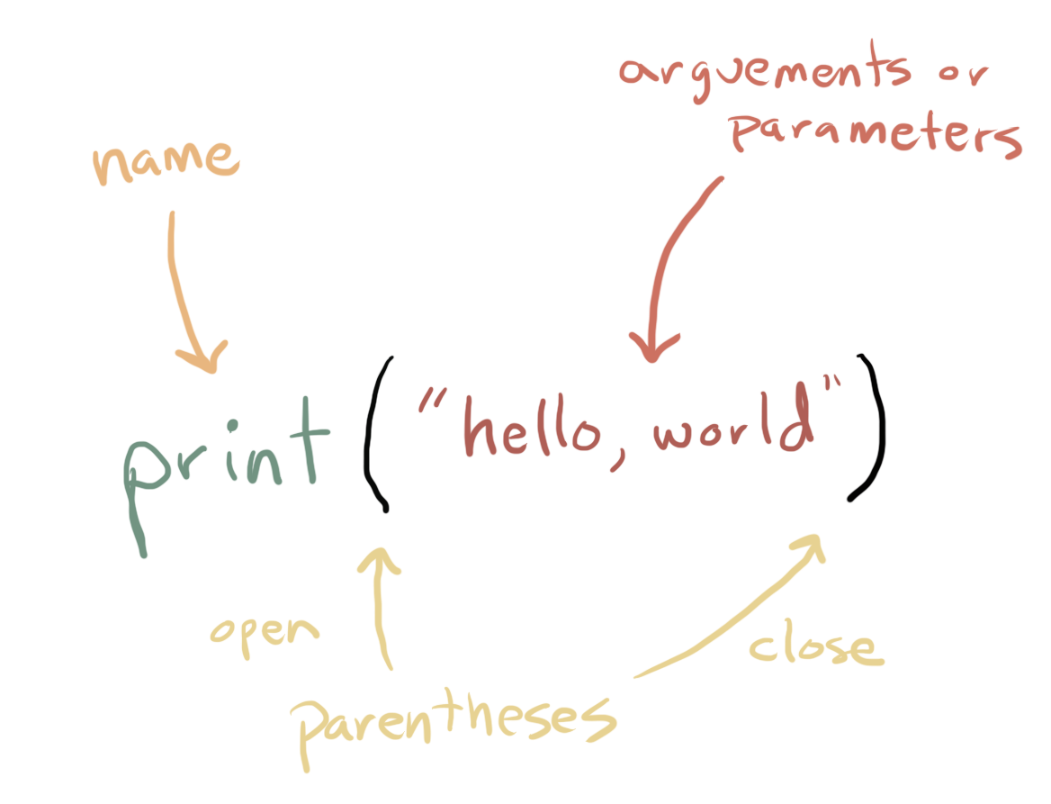
Functions have a couple of key elements:
A name which is how you specify the function you want to use
The name is followed by a open and close parentheses
()optionally, a function can include one or more arguments or parameters which are placed inside the parentheses
Here is a little schematic of how it looks:
We already say one function, which you will use a lot, called print(). The print() function lets you print out the value of whatever you provide as arguments or parameters. For example:
a=1
print(a)
1
This code defines a variable (see below) named and then prints the value of a. Notice how in Jupyter the color of the word print is special (usually green). The print() function is itself a set of lower-level commands that determine how to print things out.
Here’s another example built-in function called abs() that computes the absolute value of a number:
abs(2)
2
abs(-1)
1
Again notice the syntax here. A name for the function, and then arguments as a matched parentheses (). It is important that the parantheses are matched. If you forget the closing parentheses, you’ll get an error:
abs(1
  File "<ipython-input-8-bc02591c6df4>", line 1
    abs(1
         ^
SyntaxError: unexpected EOF while parsing
abs(-1(
  File "<ipython-input-9-bb8c754202f6>", line 1
    abs(-1(
           ^
SyntaxError: unexpected EOF while parsing
You’ll learn more about writing your own functions as well as importing other special, powerful function later. However, first I just want you to be able to pick out when a function is being used and what that looks like in the code.
4.6. Using Python as a Calculator
The Python interpreter can act as a simple calculator: type an expression at it outputs the value.
Expression syntax is straightforward: the operators +, -, * and / work just like in most other programming languages (such as Pascal or C); parentheses (()) can be used for grouping and order or precedence. For example:
2 + 2
4
50 - 5*6
20
You often have to use parentheses to enforce the order of operations.
(50 - 5*6) / 4
5.0
In most computer programming language, there are multiple “types” of numbers. This is because the internals of the computer deal with numbers differently depending on whether or not they have decimals. Specifically, the two types of numbers are: Integers (int; numbers without decimcals) or Floating-point numbers (float; numbers with decimals). You can check the type of a number using the type() function.
type(2)
int
type(2.0)
float
type(2.)
float
type(1.234)
float
Where it can sometimes get tricky is if you convert between types. For instance dividing two numbers sometimes results in a fraction result which converts the numbers to a float
8 / 5 # Division always returns a floating point number.
1.6
type(8), type(5), type(8/5)
(int, int, float)
To do what is known as a floor division and get an integer result (discarding any fractional result), you can use the // operator; to calculate the remainder, you can use %:
17 / 3 # Classic division returns a float.
5.666666666666667
17 // 3 # Floor division discards the fractional part.
5
17 % 3 # The % operator returns the remainder of the division.
2
This last operation (%) is pretty common or useful. For example, you can use it to cycle through a list of numbers:
numbers = [0,1,2,3,4,5,6,7,8,9,10]
for i in numbers:
    print(i, i%3)
0 0
1 1
2 2
3 0
4 1
5 2
6 0
7 1
8 2
9 0
10 1
Although we haven’t talked about for loops (coming below), the important thing to notice here is how we are stepping through the list of numbers between 0 and 10, but the second column of numbers is limited to between 0 and 2. Thus if you % (mod) a integer, it can create a cycle of integers between a particular value. Try changing the denominator to 5 instead of 3 and see what changes!
Other calculator type functions are ** operator to calculate powers:
5 ** 2 # 5 squared
25
2 ** 7 # 2 to the power of 7
128
In addition to int and float, Python supports other types of numbers, such as Decimal and Fraction. Python also has built-in support for complex numbers, and uses the j or J suffix to indicate the imaginary part (e.g. 3+5j).
4.7. Variables
One of the most important concepts in programming, and one feature that makes it really useful is the ability to create variables to refer to numbers. Variables are named entities that refer to certain types of data inside the programming language. We can assign values to a variable in order to save a result or use it later.
I like to think of variables as buckets.
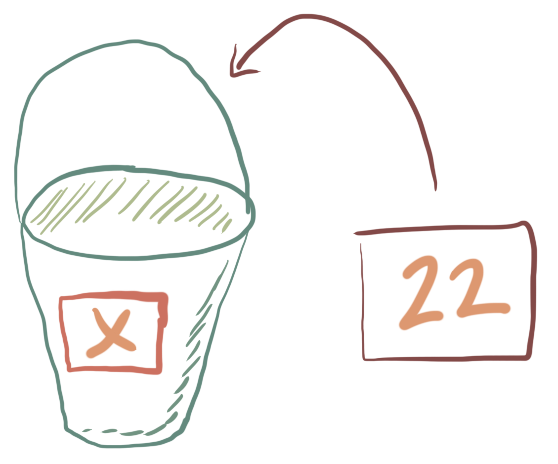
We write the name of the variable on the outside of the bucket and put something in the bucket using assignment.
Let’s look at an example. We can create a variable named width and height. The equal sign (=) assigns a value to a variable:
width = 20
height = 5 * 90
area = width * height
print("area = ", area)
area = 9000
Luckily in Python, the first time we assign something to a variable, it is created. So by executing width=20, it created in the memory of the computer a variable names width that contained the int value 20. Similarly, we created a variable called height which contains the value 5*90. Then we created a variable area which is the multiplication of width and height. One nice feature of this is that the code is kind of “readable”. By giving names to the numbers we give them meaning. We understand that this calculation computes the area of a rectangle and which dimensions refer to which parts of the rectangle.
We can make up any name for variable, but there are a few simple rules. The rules for the names of variables in Python are:
A variable name must start with a letter or the underscore character (e.g.,
_width)A variable name cannot start with a number
A variable name can only contain alpha-numeric characters and underscores (A-z, 0-9, and _ )
Variable names are case-sensitive (
age,Age, andAGEare three different variables)
Accessing the value of an undefined variable will cause an error. For instance we have not yet defined n, so asking Jupyter to output its value here will not work:
n # Try to access an undefined variable.
---------------------------------------------------------------------------
NameError                                 Traceback (most recent call last)
<ipython-input-31-2d383632fd8e> in <module>()
----> 1 n  # Try to access an undefined variable.

NameError: name 'n' is not defined
We can get a list of all the current named variables in our Jupyter kernel using this %whos command, which is a special feature of Jupyter and not part of Python core language:
%whos
Variable   Type      Data/Info
------------------------------
area       int       9000
autopep8   module    <module 'autopep8' from '<...>te-packages/autopep8.py'>
height     int       450
i          int       10
json       module    <module 'json' from '/usr<...>hon3.7/json/__init__.py'>
numbers    list      n=11
spam       int       1
text       str       # This is not a comment b<...>cause it's inside quotes.
width      int       20
You might see a number of variables here in the list but it should include the variables area, width, and height which we defined at the start of this subsection.
Variables can hold all types of information, not just single number as we will see. In fact, when we get into data analysis, we will read in entire datasets into a variable, and our graphs, statistical tests, and results will all be placed into variables. So it is good to understand the concept of variables and the rules for naming them.
Variables can also be used temporarily to move things around. For instance, let’s define variables x and y.
x = 2
y = 7
We would like to swap the values, so that x has the value of y and y has the value of x. To do this, we need to stay organized because if we just assign the value of y directly to x, it will overwrite it. So instead we will create a third “temporary” variable to swap them:
tmp = x
x = y
y = tmp
print("x = ", x)
print("y = ", y)
x =  1
y =  2
To save space in Python, you can define multiple variables at once on the same line:
width, height = 10, 20
print("width = ", width)
print("height = ", height)
10 20
This type of compact notation can even be used to more efficiently swap variables:
x, y = 1, 2
x, y = y, x
print("x = ", x)
print("y = ", y)
x =  2
y =  1
4.8. Messing with text (i.e., strings)
Besides numbers, Python can also manipulate strings. Strings are small pieces of text that can be manipulated in Python. Strings can be enclosed in single quotes ('...') or double quotes ("...") with the same result. Use \ to escape quotes, that is, to use a quote within the string itself:
'spam eggs' # Single quotes.
'spam eggs'
'doesn\'t' # Use \' to escape the single quote...
"doesn't"
"doesn't" # ...or use double quotes instead.
"doesn't"
In the interactive interpreter and Jupyter notebooks, the output string is enclosed in quotes and special characters are escaped with backslashes. Although this output sometimes looks different from the input (the enclosing quotes could change), the two strings are equivalent. The string is enclosed in double quotes if the string contains a single quote and no double quotes; otherwise, it’s enclosed in single quotes. The print() function produces a more readable output by omitting the enclosing quotes and by printing escaped and special characters:
'"Isn\'t," she said.'
'"Isn\'t," she said.'
print('"Isn\'t," she said.')
"Isn't," she said.
s = 'First line.\nSecond line.'  # \n means newline.
s  # Without print(), \n is included in the output.
'First line.\nSecond line.'
print(s) # With print(), \n produces a new line.
First line.
Second line.
String literals can span multiple lines and are delineated by triple-quotes: """...""" or '''...'''. End of lines are automatically included in the string, but it’s possible to prevent this by adding a \ at the end of the line. For example, without a \, the following example includes an extra line at the beginning of the output:
print("""
Usage: thingy [OPTIONS]
     -h                        Display this usage message
     -H hostname               Hostname to connect to
""")
Usage: thingy [OPTIONS]
     -h                        Display this usage message
     -H hostname               Hostname to connect to
Strings can be concatenated (glued together) with the + operator, and repeated with *:
# 3 times 'un', followed by 'ium'
3 * 'un' + 'ium'
'unununium'
To concatenate variables, or a variable and a literal, use +:
prefix = 'Py'
prefix + 'thon'
'Python'
Strings can be indexed (subscripted), with the first character having index 0. There is no separate character type; a character is simply a string of size one:
word = 'Python'
word[0]  # Character in position 0.
'P'
word[5] # Character in position 5.
'n'
Indices may also be negative numbers, which means to start counting from the end of the string. Note that because -0 is the same as 0, negative indices start from -1:
word[-1] # Last character.
'n'
word[-2] # Second-last character.
'o'
In addition to indexing, which extracts individual characters, Python also supports slicing, which extracts a substring. To slide, you indicate a range in the format start:end, where the start position is included but the end position is excluded:
word[0:2] # Characters from position 0 (included) to 2 (excluded).
'Py'
If you omit either position, the default start position is 0 and the default end is the length of the string:
word[:2] # Character from the beginning to position 2 (excluded).
'Py'
word[4:] # Characters from position 4 (included) to the end.
'on'
word[-2:] # Characters from the second-last (included) to the end.
'on'
This characteristic means that s[:i] + s[i:] is always equal to s:
word[:2] + word[2:]
'Python'
word[:4] + word[4:]
'Python'
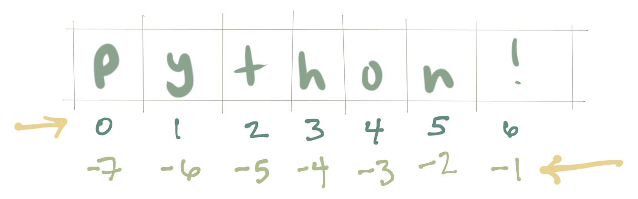
One way to remember how slices work is to think of the indices as pointing between characters, with the left edge of the first character numbered 0. Then the right edge of the last character of a string of n characters has index n. For example:
 +---+---+---+---+---+---+
 | P | y | t | h | o | n |
 +---+---+---+---+---+---+
 0   1   2   3   4   5   6
-6  -5  -4  -3  -2  -1
The first row of numbers gives the position of the indices 0…6 in the string; the second row gives the corresponding negative indices. The slice from i to j consists of all characters between the edges labeled i and j, respectively.
For non-negative indices, the length of a slice is the difference of the indices, if both are within bounds. For example, the length of word[1:3] is 2.
Attempting to use an index that is too large results in an error:
word[42] # The word only has 6 characters.
---------------------------------------------------------------------------
IndexError                                Traceback (most recent call last)
<ipython-input-68-e894f93573ea> in <module>()
----> 1 word[42]  # The word only has 6 characters.

IndexError: string index out of range
Python strings are immutable, which means they cannot be changed. Therefore, assigning a value to an indexed position in a string results in an error:
word[0] = 'J'
---------------------------------------------------------------------------
TypeError                                 Traceback (most recent call last)
<ipython-input-69-91a956888ca7> in <module>()
----> 1 word[0] = 'J'

TypeError: 'str' object does not support item assignment
The built-in function len() returns the length of a string:
s = 'supercalifragilisticexpialidocious'
len(s)
34
A couple of other useful things for strings are changing to upper or lower case:
s = 'Python'
s.upper()
'PYTHON'
s.lower()
'python'
You can also test if a part of a string is inside a larger string (more on conditionals later):
'thon' in 'Python'
True
'todd' in 'Python'
False
Reverse a string
s[::-1]
'nohtyP'
Split a string into parts based on a particular character:
s = 'milk, eggs, chocolate, ice cream, bananas, cereal, coffee'
s.split(',')
['milk', ' eggs', ' chocolate', ' ice cream', ' bananas', ' cereal', ' coffee']
The above cut the string up into a smaller string each time it encountered a comma. The results is a list… speaking of!
4.8.1. Case examples
Ok so maybe you are thinking, why do I need to program with strings? Well here are a couple of use cases where string as useful.
For example, if you want to load a file from the internet you often use a string to represent the file name. This code snippet loads the welcome screen for the psiturk package. Notice how a string is used to represent the url (i.e., the thing starting ‘https’).
import urllib.request
import json

for line in urllib.request.urlopen("https://api.psiturk.org/status_msg?version=2.3"):
    message = json.loads(line.decode('utf-8'))
    print(message['status'])
https://psiturk.org
 ______   ______     __     ______   __  __     ______     __  __
/\  == \ /\  ___\   /\ \   /\__  _\ /\ \/\ \   /\  == \   /\ \/ /
\ \  _-/ \ \___  \  \ \ \  \/_/\ \/ \ \ \_\ \  \ \  __<   \ \  _"-.
 \ \_\    \/\_____\  \ \_\    \ \_\  \ \_____\  \ \_\ \_\  \ \_\ \_\
  \/_/     \/_____/   \/_/     \/_/   \/_____/   \/_/ /_/   \/_/\/_/

             an open platform for science on Amazon Mechanical Turk

--------------------------------------------------------------------
System status:

Hi all, You need to be running psiTurk version >= 2.0.0 to use the
Ad Server feature!

The latest stable version is 2.3.0.

**ALERT**: Due to a recent Amazon API deprecation, you need to install psiturk version 2.3.0 or later.

Check https://github.com/NYUCCL/psiTurk or https://psiturk.org for
latest info.
4.9. Collections
Everything we have considered so far is mostly single elements (numbers, strings). However, we often also need to deal with collections of numbers and things (actually a string is pretty much a collection of individual characters, but…). There are three built-in types of collections that are useful to know about for this class: lists, dictionaries, and sets.
4.9.1. Lists
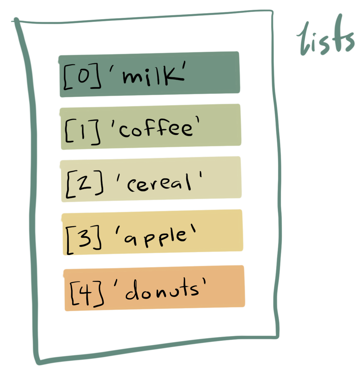
Python knows a number of compound data types, which are used to group together other values. The most versatile is the list, which can be written as a sequence of comma-separated values (items) between square brackets. Lists might contain items of different types, but usually the items all have the same type.
Here is an empty list that contains nothing:
squares = []
squares
[]
Here is a list of numbers
squares = [1, 4, 9, 16, 25]
squares
[1, 4, 9, 16, 25]
and here are two lists of either all strings or a mixture of numbers and strings:
squares_string = ["one", "four", "nine", "sixteen", "twentyfive"]
squares_string
['one', 'four', 'nine', 'sixteen', 'twentyfive']
squares_mixed = ["one", 4, 9, "sixteen", 25]
squares_mixed
['one', 4, 9, 'sixteen', 25]
Like strings (and all other built-in sequence types), lists can be indexed and sliced:
squares[0] # Indexing returns the item.
1
squares[-1]
25
squares[-3:] # Slicing returns a new list.
[9, 16, 25]
All slice operations return a new list containing the requested elements. This means that the following slice returns a new (shallow) copy of the list:
squares[:]
[1, 4, 9, 16, 25]
Lists also support concatenation with the + operator:
squares + [36, 49, 64, 81, 100]
[1, 4, 9, 16, 25, 36, 49, 64, 81, 100]
Unlike strings, which are immutable, lists are a mutable type, which means you can change any value in the list:
cubes = [1, 8, 27, 65, 125]  # Something's wrong here ...
4 ** 3  # the cube of 4 is 64, not 65!
64
cubes[3] = 64  # Replace the wrong value.
cubes
[1, 8, 27, 64, 125]
Use the list’s append() method to add new items to the end of the list:
cubes.append(216)  # Add the cube of 6 ...
cubes.append(7 ** 3)  # and the cube of 7.
cubes
[1, 8, 27, 64, 125, 216, 343]
You can even assign to slices, which can change the size of the list or clear it entirely:
letters = ['a', 'b', 'c', 'd', 'e', 'f', 'g']
letters
['a', 'b', 'c', 'd', 'e', 'f', 'g']
# Replace some values.
letters[2:5] = ['C', 'D', 'E']
letters
['a', 'b', 'C', 'D', 'E', 'f', 'g']
# Now remove them.
letters[2:5] = []
letters
['a', 'b', 'f', 'g']
# Clear the list by replacing all the elements with an empty list.
letters[:] = []
letters
[]
The built-in len() function also applies to lists:
letters = ['a', 'b', 'c', 'd']
len(letters)
4
You can nest lists, which means to create lists that contain other lists. For example:
a = ['a', 'b', 'c']
n = [1, 2, 3]
x = [a, n]
x
[['a', 'b', 'c'], [1, 2, 3]]
x[0]
['a', 'b', 'c']
x[0][1]
'b'
You can create lists from scratch using a number of methods. For example, to create a list of the number from 0 to 10, you can use the range() function which automatically generates an iterator which steps through a set of values:
list(range(10))
[0, 1, 2, 3, 4, 5, 6, 7, 8, 9]
You can also create lists by repeating a list many times:
[1]*10
[1, 1, 1, 1, 1, 1, 1, 1, 1, 1]
[0]*10
[0, 0, 0, 0, 0, 0, 0, 0, 0, 0]
[1,2]*10
[1, 2, 1, 2, 1, 2, 1, 2, 1, 2, 1, 2, 1, 2, 1, 2, 1, 2, 1, 2]
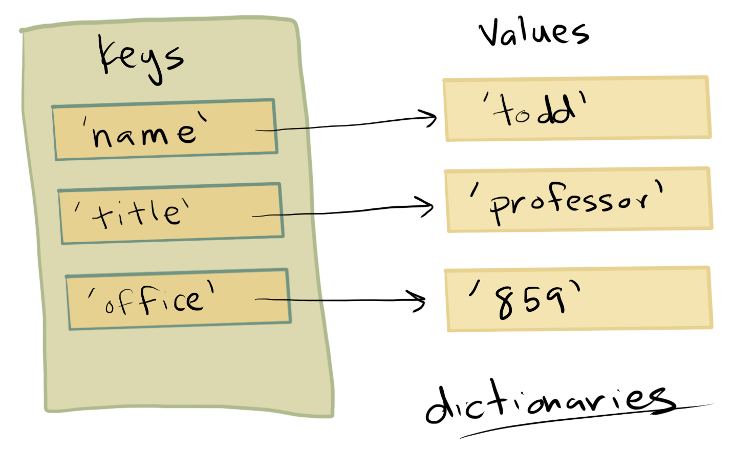
4.9.2. Dictionaries
Dictionaries are collections of key-value pairs. One easy way to understand the difference between lists and dictionaries is that in a list you can “lookup” an entry of the list using a index value (e.g., squares[1]). In a dictionary, you can look up values using anything as the index value, including string, numbers, or other Python elements (technically any object which is hashable).
First we can create an empty dictionary that contains nothing:
person = {}
Next, we might want to try initializing with some key value pairs. Each key-value pair is separate by commas (similar to a list collection) but the key and value are separated with :
person = { 'firstname': 'todd', 'lastname': 'gureckis', 'office': 859, 'hair': 'greying'}
person
{'firstname': 'todd',
 'hair': 'greying',
 'lastname': 'gureckis',
 'office': '859'}
Another way to create a dictionary is using the dict() function:
person = dict(firstname='todd', lastname='gureckis', office=859, hair='greying')
person
{'firstname': 'todd', 'hair': 'greying', 'lastname': 'gureckis', 'office': 859}
The main think about dictionaries is that you can “lookup” any value you want by the “key”:
person['firstname']
'todd'
person['hair']
'greying'
Sometimes you want to look inside a dictionary to see all the elements:
This is all the keys:
person.keys()
dict_keys(['firstname', 'lastname', 'office', 'hair'])
Values:
person.values()
dict_values(['todd', 'gureckis', 859, 'greying'])
or items:
person.items()
dict_items([('firstname', 'todd'), ('lastname', 'gureckis'), ('office', 859), ('hair', 'greying')])
Looking up a key that doesn’t exists in the dictionary results in a KeyError error:
print(person['nope'])
---------------------------------------------------------------------------
KeyError                                  Traceback (most recent call last)
<ipython-input-146-683b3d281e72> in <module>()
----> 1 print(person['nope'])

KeyError: 'nope'
In addition to initializing a dictionary you can add to it later:
person = { 'firstname': 'todd', 'lastname': 'gureckis', 'office': 859, 'hair': 'greying'}
person['age']='>30'
person['position']='associate professor'
person['building']='meyer'
person['email']='no thanks'
person
{'age': '>30',
 'building': 'meyer',
 'email': 'no thanks',
 'firstname': 'todd',
 'hair': 'greying',
 'lastname': 'gureckis',
 'office': 859,
 'position': 'associate professor'}
You can also overwrite an existing value:
person['firstname']='TODD'
person
{'age': '>30',
 'building': 'meyer',
 'email': 'no thanks',
 'firstname': 'TODD',
 'hair': 'greying',
 'lastname': 'gureckis',
 'office': 859,
 'position': 'associate professor'}
In addition to indexing by key using the [], you can use the .get() function to lookup by a key. This is useful because you can provide an optional value in case the lookup fails:
# this works
person.get('firstname')
'TODD'
# this fails but you get to return 'oops' in that case instead of an error
person.get('phonenumber', 'oops')
'oops'
You can merge two dictionary together:
dict1 = {'a': 1, 'b': 2}
dict2 = {'c': 3}
dict1.update(dict2)
print(dict1)
{'a': 1, 'b': 2, 'c': 3}
If they have the same keys, the second one will overwrite the first.
# If they have same keys:
dict1.update({'c': 4})
print(dict1)
{'a': 1, 'b': 2, 'c': 4}
Why learn about dictionaries? Well at least one reason is that dictionaries are a very useful way of organizing data. For example, one might naturally think of the columns of a excel spreadsheet or data file as being labeled with ‘keys’ that have a list of values underneath them. This is exactly a data format that pandas (a library that we will use in this class; more on this and other libraries later) likes:
import pandas as pd
df=pd.DataFrame({'student': [1,2,3,4], 'grades':[0.95, 0.27, 0.45, 0.8] })
df
| student | grades | |
|---|---|---|
| 0 | 1 | 0.95 |
| 1 | 2 | 0.27 |
| 2 | 3 | 0.45 |
| 3 | 4 | 0.80 |
Another reason is that a very common data file format online is JSON, which is a data file format composed of key-value pairs. Here is an example of a string that contains JSON:
jsonstring='''
{
     "firstName": "John",
     "lastName": "Smith",
     "address": {
         "streetAddress": "21 2nd Street",
         "city": "New York",
         "state": "NY",
         "postalCode": 10021
     },
     "phoneNumbers": [
         "212 555-1234",
         "646 555-4567"
     ]
 }
'''
Which can be quickly loaded into a dictionary using the json library:
import json
json_dictionary=json.loads(jsonstring)
json_dictionary
{'address': {'city': 'New York',
  'postalCode': 10021,
  'state': 'NY',
  'streetAddress': '21 2nd Street'},
 'firstName': 'John',
 'lastName': 'Smith',
 'phoneNumbers': ['212 555-1234', '646 555-4567']}
json_dictionary['firstName']
'John'
json_dictionary['phoneNumbers']
['212 555-1234', '646 555-4567']
json_dictionary['address']
{'city': 'New York',
 'postalCode': 10021,
 'state': 'NY',
 'streetAddress': '21 2nd Street'}
This last example shows how a dictionary can be inside a dictionary!
4.9.3. Sets
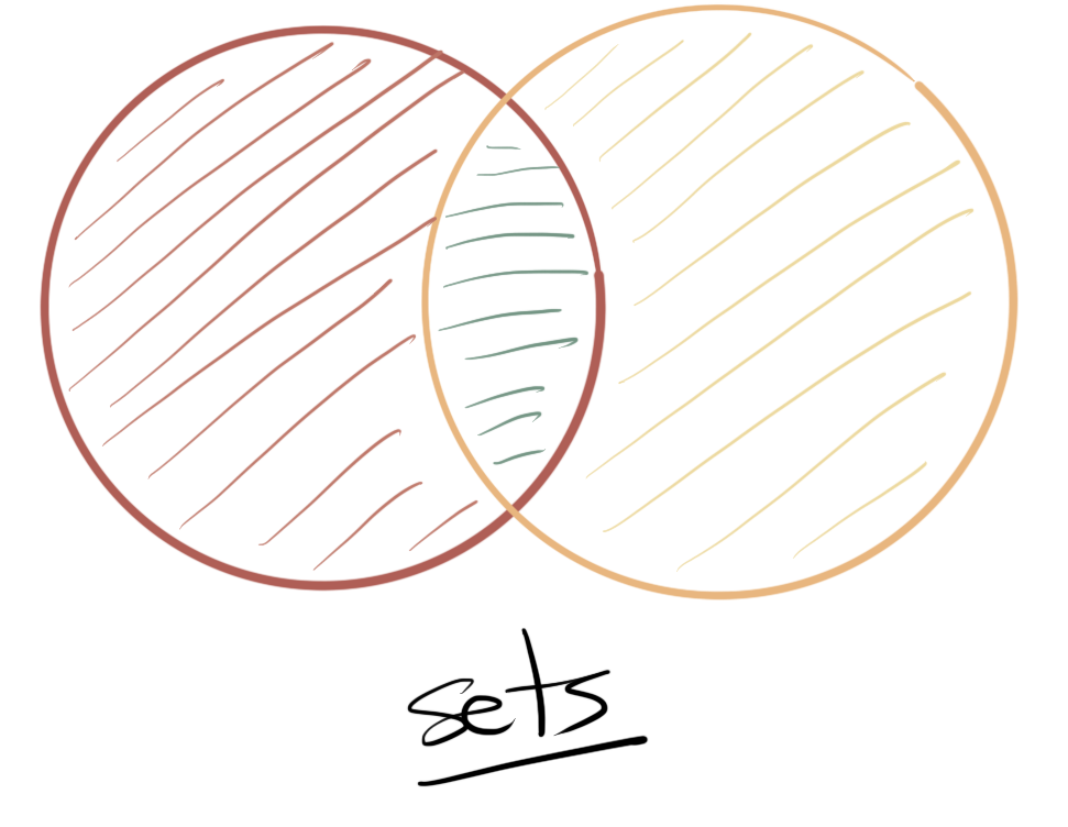
The final collection we will discuss is a set. You might have learned about sets and set theory in high school. Well Python has some tools for reasoning about sets. Remember a set is an unordered collection of objects. So unlike a list, there is not “first element” or “second element” in a set. Instead, a set just contains objects and allows you to do various types of set operations, such as testing if an element is within a set, testing if a set is a subset of another set, etc…
You can create a set like this:
animal_set = set(['Coyote', 'Dog', 'Bear', 'Cat', 'Elephant'])
animal_set
{'Bear', 'Cat', 'Coyote', 'Dog', 'Elephant'}
Notice how even though ‘Coyote’ was the first element in the list that we used to initialize the set, it is no longer the first item in the output. This is because sets are unordered.
Sets are related to dictionaries (the elements of a dictionary are also unordered but they are indexed by a key where as a set has no key). Thus, you can create a set using the {} operations.
set_1 = {2, 4, 6, 8, 10}
set_2 = {42, 'foo', (1, 2, 3), 3.14159}
print(type(set_1))
<class 'set'>
The size of a set can be found with the len() operator we saw before:
len(animal_set)
5
You can test if an element is contained within a set:
'owl' in animal_set
False
'Coyote' in animal_set
True
You can take the union of two sets, which will find all the elements unique and in common to both set. Repeats are removed this way:
x1 = {'foo', 'bar', 'baz'}
x2 = {'baz', 'qux', 'quux'}

x1 | x2
{'bar', 'baz', 'foo', 'quux', 'qux'}
# or
x1.union(x2)
{'bar', 'baz', 'foo', 'quux', 'qux'}
You can also find the set intersection
x1 = {'foo', 'bar', 'baz'}
x2 = {'baz', 'qux', 'quux'}

x1.intersection(x2)
{'baz'}
x1 & x2
{'baz'}
The intersection finds the things in one set that are not in the other:
x1 = {'foo', 'bar', 'baz'}
x2 = {'baz', 'qux', 'quux'}

x1.difference(x2)
{'bar', 'foo'}
x1-x2
{'bar', 'foo'}
The symmetric_difference function finds the things in either set A or set B but not both:
x1 = {'foo', 'bar', 'baz'}
x2 = {'baz', 'qux', 'quux'}

x1.symmetric_difference(x2)
{'bar', 'foo', 'quux', 'qux'}
x1 ^ x2
{'bar', 'foo', 'quux', 'qux'}
You and ask if two sets contain anything in common using isdisjoint().
x1 = {1, 3, 5}
x2 = {2, 4, 6}

x1.isdisjoint(x2)
True
x1 = {1, 3, 5, 7} # adding one element in commont
x2 = {2, 4, 6, 7}

x1.isdisjoint(x2)
False
You can ask if one set is a subset of another one:
x1 = {1, 3, 5, 7}
x2 = {2, 4, 6, 7}

x1.issubset(x2)
False
x1 = {2,4}
x2 = {2, 4, 6, 7}

x1.issubset(x2)
True
To add or remove a new element to the set, just use add() or remove()
x1.add('foo')
x1
{2, 4, 'foo'}
x1.remove('foo')
x1
{2, 4}
Sets are sometimes useful in data analysis because they can be used to get all the unique elements of a list. For example, if you have a list of ages of participants, a set could be a nice way to find the different values it takes:
ages = [14,15,35,15,24,14,17,18,22,22,24]
set(ages)
{14, 15, 17, 18, 22, 24, 35}
len(set(ages))
7
The above shows there are 7 unique ages in the data set by getting rid of duplicates.
4.10. Flow Control
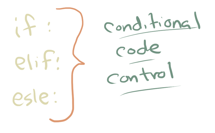
Within a Jupyter code cell, we have been seeing each line of code execute in sequence. However often times we need to exert control over which bits of code run depending on other variables or settings. The is generally known as flow control elements. These include conditionals like if, else, and elif, as well as loops like for. Again this is not a full programming course so we can only cover this in partial depth (e.g., we will not talk about while loops although they can be really useful). However, it should be enough to get by in this class.
4.10.1. Testing if things are true
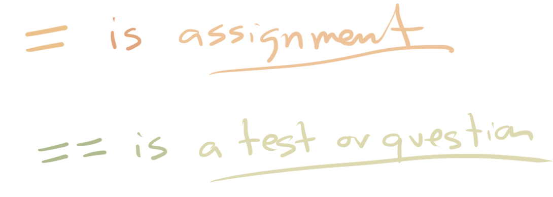
The first thing we need is to consider how we deal with testing if some condition has been met. One of the most common ways to deal with this in Python is with the double equals sign ==. The double equals sign is different from the single equals sign in that the single assign a value to a variable while the double tests if two things are equal or not. Thus the single equal sign is a bit like a command to “make these things equal” whereas the double equal sign is a bit more like a question asking “are these two things equal?”
1==2
False
1==1
True
'hello'=='hello'
True
'hello'=='HELLO'
False
While this gives you a few example, a more common use case is testing if a variable is equal to a particular value. We already know 1 is equal to 1, but we might not know the contents of a variable and thus testing gives us a way to check if it means a particular condition.
myvar = 10

myvar == 10
True
myvar == 11
False
There are related comparisons. For example, we might want to test if a variable is greater than a particular value
myvar > 10 # is myvar greater than 10
False
myvar >=5 # is myvar greater than or equal to 5
True
myvar <= 15 # is myvar less than or equal to 15
True
A final one is not equal to which is just the opposite of the ==:
myvar != 5
True
myvar != 10
False
There is also a slightly more English-like version of this test:
myvar is 10
True
myvar is not 10
False
We can also test if an item is a part of a collection (e.g., a list or set):
mylist = ['one', 'two', 'three', 'four']

'one' in mylist # is 'one' in mylist?
True
'six' not in mylist # is 'six' not in mylist?
True
mystring = 'lkjasldfkj'

'jas' in mystring # tests if 'jas' is a substring of mystring
True
'jas' not in mystring # tests if 'jas' is not a substring of mystring
False
4.10.2. Conditionals (if-then-else)
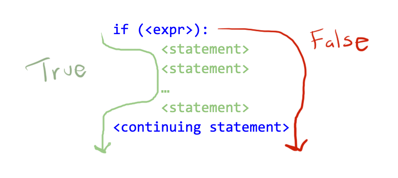
Now that we have seen a few ways to test if things are true/false or meet some particular condiiton, the next step is to execute different code depending on what the test gives us. The simplest version of code that accomplishes this has the general form like this:
if <expression>:
    <code block>
where expression is a true/false (Boolean) as described in the previous section and <code block> is some collection of lines that will be executed only if the expression is True.
For a more example, lets create a variable called ‘myvar’ and set it equal to 10. Then we will write a short program that prints ‘hi’:
weather = 'nice'

if weather == 'nice':
    print('Walk the dog')
    print('Mow the lawn')
    print('Weed the flower bed')
Mow the lawn
Weed the garden
Walk the dog
The important thing about this code is that you could run it even if you weren’t sure what the value of weather was because it was set earlier in the program or by some other piece of complex code. Thus, it lets you run a special bit of code depending on the value of a variable.
The situation you would use this type of code in is very intuitive… sometimes you only do certain step when something is true (like take an umbrella when it is raining).
Now there is a couple of very important but sometimes subtle or confusing parts about this.
First is that you’ll notice that the lines which reads print() are not aligned with the rest of the code in that cell. This is because the first character of that line is the tab character (the one on your keyboard you sometimes use to start the first line of a paragraph when writing).
In Python this spacing is very important. Any line that is tabbed over from the line above it is known as a “code block”:
myvar = 10
myvar2 = 20

if myvar == myvar2:
    # this is inside the code block
    print("this is")
    print("a code block")

# this is not in the code block because it is not tabbed over
print("this is not")
this is not
All programming languages have some type of code block syntax, but in Python, you just use tab and untab to do this. This feature might actually be one of the main reasons Python is so popular (I kid you not). The reason is this is a very elegant way to indicate code blocks and it makes the code very readable compared to other languages. The simplicity can sometimes be confusing for new users, though, because you really have to keep track of the level of indentation of your code. It is not a big deal once you get used to it but at first you will need to be on-guard about which lines are or are not tabbed over.
myvar = 10
myvar2 = 10

if myvar == myvar2:
    print("this is")
    print("a code block")

print("this is not")
this is
a code block
this is not
Consider the two contrasting examples above (the one just now and the one before it). In one, myvar and myvar2 have a different value. Thus, the equal == test fails (return False) and then the tabbed code block is skipped. In the second example, the value of the test is True so the code block is run. In both cases, the final print (which is not tabbed over) runs no matter what (so it is printed out in both examples). The general structure is this:
In the if statement we just considered you take an optional path through the code and then continue. However, othertimes you want to take one path if something is True and another path if it is False. For example:
if raining:
   - take umbrella
otherwise:
   - take sunglasses
- take wallet
This is not valid Python but it makes intuitive sense… sometimes if the conditional is false we want to do something else. This in Python is accomplished with the else command:
raining = True

if raining:
    print("Take umbrella")
else:
    print("Take sunglasses")

print("Take wallet")
Take umbrella
Take wallet
raining = False

if raining:
    print("Take umbrella")
else:
    print("Take sunglasses")

print("Take wallet")
Take sunglasses
Take wallet
If you compare the two code cells above, you can see that depending on the value of raining (either True or False… these are special words in Python) then it takes a different path through the code.
Great, but what if there many conditions? So you might want to take your sunglasses only if it is not cloudy. But somedays it might not be raining but still be cloudy and so you can use the elif (which is a combination of the else and if commands to consider multiple conditions:
weather = 'sunny'

if weather == 'raining':
    print("Take umbrella")
elif weather == 'sunny':
    print("Take sunglasses")
elif weather == 'cloudy':
    print("Take sweater")

print("Take wallet")
Take sunglasses
Take wallet
weather = 'raining'

if weather == 'raining':
    print("Take umbrella")
elif weather == 'sunny':
    print("Take sunglasses")
elif weather == 'cloudy':
    print("Take sweater")

print("Take wallet")
Take umbrella
Take wallet
weather = 'cloudy'

if weather == 'raining':
    print("Take umbrella")
elif weather == 'sunny':
    print("Take sunglasses")
elif weather == 'cloudy':
    print("Take sweater")

print("Take wallet")
Take sweater
Take wallet
Comparing the three cells above, you can see that depending on multiple values that the variable weather could take, you do different things. Pretty simple!
If needed, you can always end a if/elif sequence with an final else:
weather = 'heat wave'

if weather == 'raining':
    print("Take umbrella")
elif weather == 'sunny':
    print("Take sunglasses")
elif weather == 'cloudy':
    print("Take sweater")
else:
    print("I don't know what to do!")

print("Take wallet")
I don't know what to do!
Take wallet
Here, in the case we come up against a heat wave (or anything else!), our program doesn’t know what to recommend!
4.10.3. For Loops
Using loops in computer programming allows us to automate and repeat similar tasks multiple times. This is very common in data analysis. In this tutorial, we’ll be covering Python’s for loop.
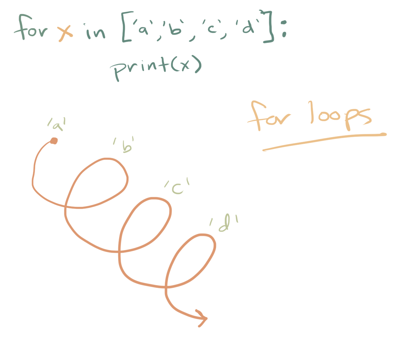
A for loop implements the repeated execution of code based on a loop counter or loop variable. This means that for loops are used most often when the number of repetitions is known before entering the loop, unlike while loops, which can run until some condition is met.
In Python, for loops are constructed like so:
for [iterating variable] in [sequence]:
    [do something]
The something that is being done (known as a code block) will be executed until the sequence is over. The code block itself can consist of any number of lines of code, as long as they are tabbed over once from the left hand side of the code.
Let’s look at a for loop that iterates through a range of values:
for i in range(0,5):
   print(i)
0
1
2
3
4
This for loop sets up i as its iterating variable, and the sequence exists in the range of 0 to 5.
Then within the loop, we print out one integer per loop iteration. Keep in mind that in programming, we tend to begin at index 0, so that is why although 5 numbers are printed out, they range from 0-4.
You’ll commonly see and use for loops when a program needs to repeat a block of code a number of times.
4.10.3.1. For Loops using range()
One of Python’s built-in immutable sequence types is range(). In loops, range() is used to control how many times the loop will be repeated.
When working with range(), you can pass between 1 and 3 integer arguments to it:
startstates the integer value at which the sequence begins, if this is not included then start begins at 0stopis always required and is the integer that is counted up to but not includedstepsets how much to increase (or decrease in the case of negative numbers) the next iteration, if this is omitted then step defaults to 1
We’ll look at some examples of passing different arguments to range().
First, let’s only pass the stop argument, so that our sequence set up is range(stop):
for i in range(6):
   print(i)
0
1
2
3
4
5
In the program above, the stop argument is 6, so the code will iterate from 0-6 (exclusive of 6).
Next, we’ll look at range(start, stop), with values passed for when the iteration should start and for when it should stop. Here, the range goes from 20 (inclusive) to 25 (exclusive), so the output looks like this:
for i in range(20,25):
    print(i)
20
21
22
23
24
The step argument of range() can be used to skip values within the sequence.
With all three arguments, step comes in the final position: range(start, stop, step). First, let’s use a step with a positive value. In this case, the for loop is set up so that the numbers from 0 to 15 print out, but at a step of 3, so that only every third number is printed, like so:
for i in range(0,15,3):
   print(i)
0
3
6
9
12
We can also use a negative value for our step argument to iterate backwards, but we’ll have to adjust our start and stop arguments accordingly. Here, 100 is the start value, 0 is the stop value, and -10 is the range, so the loop begins at 100 and ends at 0, decreasing by 10 with each iteration. We can see this occur in the output:
for i in range(100,0,-10):
   print(i)
100
90
80
70
60
50
40
30
20
10
When programming in Python, for loops often make use of the range() sequence type as its parameters for iteration.
4.10.3.2. For Loops using Sequential Data Types
Lists and other data sequence types can also be leveraged as iteration parameters in for loops. Rather than iterating through a range(), you can define a list and iterate through that list.
We’ll assign a list to a variable, and then iterate through the list:
sharks = ['hammerhead', 'great white', 'dogfish', 'frilled', 'bullhead', 'requiem']

for shark in sharks:
   print(shark)
hammerhead
great white
dogfish
frilled
bullhead
requiem
The output above shows that the for loop iterated through the list, and printed each item from the list per line.
Lists and other sequence-based data types like strings and tuples are common to use with loops because they are iterable. You can combine these data types with range() to add items to a list, for example:
sharks = ['hammerhead', 'great white', 'dogfish', 'frilled', 'bullhead', 'requiem']

for item in range(len(sharks)):
   sharks.append('shark')

print(sharks)
['hammerhead', 'great white', 'dogfish', 'frilled', 'bullhead', 'requiem', 'shark', 'shark', 'shark', 'shark', 'shark', 'shark']
Here, we have added a placeholder string of ‘shark’ for each item of the length of the sharks list.
You can also use a for loop to construct a list from scratch. In this example, the list integers is initialized as an empty list, but the for loop populates the list like so:
integers = []

for i in range(10):
   integers.append(i)

print(integers)
[0, 1, 2, 3, 4, 5, 6, 7, 8, 9]
Similarly, we can iterate through strings:
sammy = 'Sammy'

for letter in sammy:
   print(letter)
S
a
m
m
y
When iterating through a dictionary, it’s important to keep the key:value structure in mind to ensure that you are calling the correct element of the dictionary. Here is an example that calls both the key and the value:
sammy_shark = {'name': 'Sammy', 'animal': 'shark', 'color': 'blue', 'location': 'ocean'}

for key in sammy_shark:
   print(key + ': ' + sammy_shark[key])
name: Sammy
animal: shark
color: blue
location: ocean
When using dictionaries with for loops, the iterating variable corresponds to the keys of the dictionary, and dictionary_variable[iterating_variable] corresponds to the values. In the case above, the iterating variable key was used to stand for key, and sammy_shark[key] was used to stand for the values.
Loops are often used to iterate and manipulate sequential data types.
4.10.3.3. Nested For Loops
Loops can be nested in Python, as they can with other programming languages.
A nested loop is a loop that occurs within another loop, structurally similar to nested if statements. These are constructed like so:
for [first iterating variable] in [outer loop]: # Outer loop
    [do something]  # Optional
    for [second iterating variable] in [nested loop]:   # Nested loop
        [do something]
The program first encounters the outer loop, executing its first iteration. This first iteration triggers the inner, nested loop, which then runs to completion. Then the program returns back to the top of the outer loop, completing the second iteration and again triggering the nested loop. Again, the nested loop runs to completion, and the program returns back to the top of the outer loop until the sequence is complete or a break or other statement disrupts the process.
Let’s implement a nested for loop so we can take a closer look. In this example, the outer loop will iterate through a list of integers called num_list, and the inner loop will iterate through a list of strings called alpha_list.
num_list = [1, 2, 3]
alpha_list = ['a', 'b', 'c']

for number in num_list:
    print(number)
    for letter in alpha_list:
        print(letter)
1
a
b
c
2
a
b
c
3
a
b
c
The output illustrates that the program completes the first iteration of the outer loop by printing 1, which then triggers completion of the inner loop, printing a,b, c consecutively. Once the inner loop has completed, the program returns to the top of the outer loop, prints 2, then again prints the inner loop in its entirety (a, b, c), etc.
Nested for loops can be useful for iterating through items within lists composed of lists. In a list composed of lists, if we employ just one for loop, the program will output each internal list as an item:
list_of_lists = [['hammerhead', 'great white', 'dogfish'],[0, 1, 2],[9.9, 8.8, 7.7]]

for list in list_of_lists:
    print(list)
['hammerhead', 'great white', 'dogfish']
[0, 1, 2]
[9.9, 8.8, 7.7]
In order to access each individual item of the internal lists, we’ll implement a nested for loop:
list_of_lists = [['hammerhead', 'great white', 'dogfish'],[0, 1, 2],[9.9, 8.8, 7.7]]

for list in list_of_lists:
    for item in list:
        print(item)
hammerhead
great white
dogfish
0
1
2
9.9
8.8
7.7
When we utilize a nested for loop, we are able to iterate over the individual items contained in the lists.
Another useful looping structure in known as a while-loop. We don’t have time to go through a while loop in detail and they are used a bit less often in our data analysis but you can watch this great tutorial on RealPython.
On the class webpage there is also an example of 40 For loops which show many concrete examples used in data analysis that you might find helpful.
4.11. Writing New Functions
In the previous sections, we learned how we can organize code into code blocks by tabbing it over and wrapping it in control structures (which then execute the code a certain number of times or depending on some particular condition). As you begin to write longer and longer programs though, it sometimes helps to break up the functionality of your programs into reuseable chunks called functions. Functions make your code more readable, save time and typing by organizing bits of code into reuseable chunks, and make it easier to share your code with other people.
The general format for a function is composed of a few elements. First there is a line the defines the name of the function and the parameters is can take (more on that later). Next a sequence of instructions are provided that are tabbed over from the definition. Ending the tab ends the definition of the function:
def my_function(parameter1, parameter2):
    <code line 1>
    <code line 2>
    <code line 3>
This just gives you a general sense of those functions are organized and is not a valid Python command!
Let’s look at an actual version.
def my_function():
    print("Hello from my function")
Notice two things about this function. First is that is has no parameters (which is fine… we’ll talk about how to add them later). Second, when you run this code cell, nothing happens. This is because this simply defines the function but does not run it. To run this function someplace else in our code, we would write:
my_function()
Hello from my function
Here we “executed” (i.e., ran) the function by calling its name with the parentheses.
Functions can be combined with other elements of Python to create more complex program flows. For example, we can combine a custom function with a for loop:
def my_ramp():
    print('*')
    print('***')
    print('*****')

for i in range(4):
    my_ramp()
*
***
*****
*
***
*****
*
***
*****
*
***
*****
The above code, which prints out a ramping set of stars four times, is much more efficient than if you repeated the print statements 16 times.
4.11.1. Parameters
Functions can take different types of “parameters”, which are essentially variables that are created at the start of the execution of the function. This is helpful for making more abstract functions that perform some computation with their inputs. For example:
def add(x, y):
    print("The sum is ", x+y)
The add functions we just defined takes two parameters x and y. These parameters are then used as the operands to an addition operation. As a result, we can run this function many times with different inputs and get different results:
add(1,2)
The sum is 3
add(34,28)
The sum is 62
4.11.2. Return values
The functions we have considered so far simply print something out and then finish. However, sometimes you might like to have your function give back one or more result for further processing by other parts of your program. For instance, instead of printing out the sum of x and y, we can redefine the sum() function to return the sum using a special keyword return:
def sum(x,y):
    return x+y
Now when we run this function, instead of printing out a message, the value of the sum is calculated and passed back.
sum(4,5)
9
This allows you to continue to do additional processing. For example, we can add two numbers and then compute the square root of them:
import math

math.sqrt(sum(4,5))
3.0
You can return multiple values from a function if you want. For example, we could create a function call arithmetic that does a number of operations to x and y and returns them all:
def arithmetic(x,y):
    _sum = x+y
    _diff = x-y
    _prod = x*y
    _div = x/y
    return _sum, _diff, _prod, _div
This new function gives back a tuple (similar to a list) that contains all four of the results in one step.
arithmetic(7,3)
(10, 4, 21, 2.3333333333333335)
4.12. Importing additional functionality
One of the best features of Python, and one reason contributing to its popularity is the large number of add on packages. For example, there are packages for data analysis (pandas), plotting (matplotlib or seaborn), etc… These packages are not all loaded automatically. Instead at the start of your notebook or program, you often need to import this functionality. There are a couple of ways to import packages. Generally you need to know the name of the package and details about what functions or methods it provides. Most packages have tons of great documentation. For example, pandas a library we will use a lot in class has extensive documentation on the pydata website.
Basic importing is accomplished with the import command. For example, to import the back math functions in Python just type:
import math
Now we can access the methods provided by the math function using the . (dot) operator. Any function that the math library provides is accessible to us now using math.<function>. For example, to compute the cosine of a number:
math.cos(1)
0.5403023058681398
Sometimes we want to import a library but rename it so that it is easier to type. For instance we will use the pandas library a lot in class. If we type import pandas that will load the library but that means everytime we use a pandas function it will need to begin with the pandas.<something> syntax. This can be a lot of typing. As a result many popular packages are imported using the import <package> as <shortname> syntax. This imports the library but immediately changes its name, usually to something simpler and shorter for easy typing. For example it is traditional to import pandas and rename it pd. Thus to import pandas this way, we would type this at the top of our notebook or script:
import pandas as pd
Now we have access to the pandas function using pd.<something>. For example, we can create a new pandas dataframe like this:
import pandas as pd
df=pd.DataFrame({'student': [1,2,3,4], 'grades':[0.95, 0.27, 0.45, 0.8] })
df
| student | grades | |
|---|---|---|
| 0 | 1 | 0.95 |
| 1 | 2 | 0.27 |
| 2 | 3 | 0.45 |
| 3 | 4 | 0.80 |
It was a lot shorter to import pandas as pd and then call the pd.DataFrame() command than to type out pandas.DataFrame().
If you know there is a particular function you want to grab from a library, you can import only that function. For example, we could import the cos() function from the math library like this:
from math import cos
This is generally useful if there is a really large and complex library and you only need part of it for your work.
Python libraries can really extend your computing and data options. For example, one cool library is the wikipedia library which provides an interface to the Wikipedia site.
import wikipedia as wk
wk.search("Carbon Dioxide")
['Carbon dioxide',
 'Carbon dioxide scrubber',
 'List of countries by carbon dioxide emissions',
 'Carbon capture and storage',
 "Carbon dioxide in Earth's atmosphere",
 'Carbon dioxide equivalent',
 'Carbon dioxide removal',
 'Hypercapnia',
 'Carbon sequestration',
 'Carbon dioxide laser']
The search() command in the wikipedia will search all wikipedia packages that match a particular search string. Here it brings up all pages relevant to the phrase “Carbon Dioxide”.
4.13. Dealing with error messages
Often times you will run into error messages when using Python. This is totally fine! It is not a big deal and comes up all the time. In fact if you don’t make errors sometimes then you are probably not learning enough.
Most errors in python generate what is known as an “exception” where the code doesn’t necessarily “crash” but a warning is issued. For example, if we have too many parentheses (each parentheses you open must be closed by the same type of character) you will get a SyntaxError:
print(0/0))
  File "<ipython-input-3-ded43ae9deb7>", line 1
    print(0/0))
              ^
SyntaxError: invalid syntax
There are a couple of things to notice about this error. First is that it does give you some indication of what happened (for examples it say “invalid syntax” which means the code doesn’t look right to python and so it can’t understand it). It also shows you where the first error occured (here on line 1 of the cell, and it even indicates which character in that line might be the problem.) From this message you could easily fix you code simply by removing the extra parantheses at the end.
print(0/0)
---------------------------------------------------------------------------
ZeroDivisionError                         Traceback (most recent call last)
<ipython-input-4-1babb3b33639> in <module>()
----> 1 print(0/0)

ZeroDivisionError: division by zero
Ooops but this gives a different error! Not we are getting and error because we are attempting to divide by zero. Again, the messages if you read them kind of give some helpful infomation.
In most cases you can simply fix the code in your cell, try to re-run it and keep going until you get it right. However, one problem can come up in that errors compound on one another. For example, your error might have accidently renamed a variable or introduced a variable you don’t want. In that case it can be helpful to choose Kernel->Restart Kernel from the file menu. This effectively “restarts” the computing engine that you are working with and reset it to a fresh session. You will need to re-run all the cells prior to your error in that case but this is easy. There is even a shortcut on the “Cell” menu called “run all cells above” that will let you rerun everything prior to the current selected cell. This can be a great way to restart and get back to where you were working originally.
4.14. Wrapping up
This chapter has tried to give you a general overview of Python programming and many of the language features you will encounter again and again in this course. It is not all there is to learn about Python and once you get started, you can learn for years if you like. There are many excellent online resources for adding to your Python knowledge including youtube videos, free online tutorials, and even online classes. Thus, use this as a starting place for learning more about the language. However, if you are able to master the above concepts, then you shouldn’t have too much difficulty with this course.
4.15. Further Reading and Resources
This is a collection of useful python resources including videos and online tutorials. This can help student how have less familiarity with programming in general or with python specifically.
A nice, free textbook ”How to Code in Python” by Lisa Tagliaferri
CodeAcademy has a variety of courses on data analysis with Python. There is a free tutorial on Python 2.0. Although this class uses Python 3.0 and there are minor difference, a beginning programmer who didn’t want to pay for the code academy content might benefit from these tutorials on basic python syntax: Python 2.0 tutorial
Microsoft has an Introduction to Python video series. Each video is about 10 minutes long and introduces very basic python features.
A nice multi-part tutorial on Data Visualization with Python and Seaborn that gets into many more details about Seaborn than we have time to cover in class.
A six hour (free) video course on basic Python programming on youtube