Analytical Solutions of PDEs using PDEtools in Maple 

Aleksandar Donev, Courant Institute 

This is largely based on examples in the excellent Maple documentation 

>

restart:

 

The PDEtools package is a collection of commands and routines for finding analytical solutions for partial differential equations (PDEs) based on the paper "A Computational Approach for the Analytical Solving of Partial Differential Equations" by E.S. Cheb-Terrab and K. von Bulow (see References ), and the continuation of this work by the same authors ( Symmetry routines ) during 2004. 

>	with(PDEtools):

 

First-Order PDEs 

Maple knows about the method of characteristics: 

>	U := diff_table(u(x,t)): # To enable compact notation U_xx etc.

 

>	PDE := U[t]+c*U[x]=-lambda*U[]; # Advection-reaction linear equation

 

(1)

 

>	IC := eval(U[], t=0) = phi(x); # Initial conditions

 

(2)

 

>	pdsolve([PDE,IC]); # Try to solve the PDE automatically - works!

 

(3)

 

Try to get a general solution: 

>	pdsolve(PDE); # No initial condition

 

(4)

 

>	PDE := U[t]+c*U[x]=-lambda*U[]^2; # Advection-reaction nonlinear equation

 

(5)

 

>	pdsolve([PDE,IC]); # Works here also since simple first-order equation

 

(6)

 

>	PDE := U[t]+c*U[]*U[x]=0; # Burger's equation

 

(7)

 

>	pdsolve([PDE,IC]); # Does not return anything (cannot find solution)

 

Heat Equation 

>	restart: with(PDEtools):

 

Maple knows about the method of separation of variables: 

>	BVP:=[diff(u(x, t), t) = k*diff(u(x, t), x, x), u(0, t) = 0, u(Pi, t) = 0, u(x,0) = f(x)]; # Heat equation in 1D with homogeneous Dirichlet BCs

 

(8)

 

>	sol:=pdsolve(BVP);

 

(9)

 

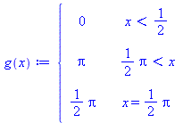
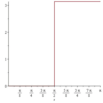
>	g(x):=piecewise(x<1/2,0,x>Pi/2,Pi,x=Pi/2,Pi/2);

 

(10)

 

>	plot(g(x),x=0..Pi)

 

>	pdsolve(eval(BVP, f(x)=g(x)));

 

Error, (in casesplit/K) this version of casesplit is not yet handling the function: piecewise

 

>	temp:=eval(sol, f(x)=g(x));

 

(11)

 

>	sol_series:=value(temp);

 

(12)

 

Numerical Evaluation 

Plotting the Solution 

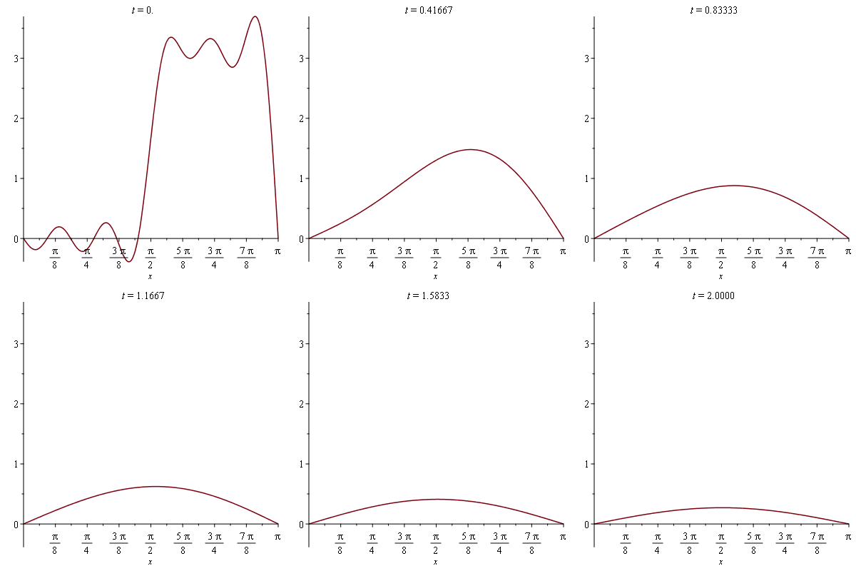
To plot this we need to truncate the sum to a few terms 

>	summand:=op(1, rhs(sol_series));

 

(13)

 

>	summand:=eval(summand, {_Z1=n, k=1});

 

(14)

 

Here we only take 10 terms: 

>	sol_approx:=unapply(simplify(add(summand, n=1..10)),t);

 

(15)

 

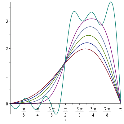
>	plot( {seq(sol_approx(i*0.05), i=0..5)}, x=0..Pi);

 

We can turn this into an animation to make it more informative: 

>	plots[animate]( plot, [sol_approx(t), x=0..Pi], t=0..2 );

 

Gibbs Phenomenon 

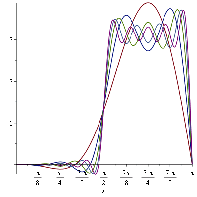
At t=0 we are getting the Gibbs phenomenon, lets explore this some more: 

>	summ0:=eval(summand, t=0);

 

(16)

 

>	plot( {seq(add(summ0, n=1..4*N), N=1..5)}, x=0..Pi);

 

Numerical Accuracy 

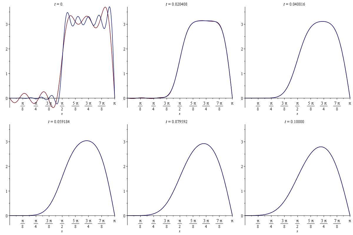
To see how good our solution is, we should really compare with the solution obtained by including more terms 

>	sol_better_approx:=unapply(simplify(add(summand, n=1..20)),t):

 

>	plots[animate]( plot, [{sol_approx(t), sol_better_approx(t)}, x=0..Pi], t=0..0.1, frames=50);

 

Wave Equation (from recitation) 

Here we try to solve  Problem 9 in section 4.7 of APDE, as was done in recitation on 4/15/2016 by recitation leader JT. Look at his solution notes first. 

>	restart: with(PDEtools):

 

>	BVP:=[diff(u(x, t), t,t) = diff(u(x, t), x, x), u(0, t) = 0, u(1, t) = sin(t), u(x,0) = x*(1-x), D[2](u)(x,0)=0];

 

(17)

 

>	#infolevel[pdsolve]:=5; # If you want to see what Maple is trying out

 

>	sol:=pdsolve(BVP); # No solution returned

 

(18)

 

Let's try to see what the problem is, inhomogeneous BCs, or initial condition, or what: 

>	BVP_hom:=[diff(u(x, t), t,t) = diff(u(x, t), x, x), u(0, t) = 0, u(1, t) = 0,  u(x,0) = x*(1-x), D[2](u)(x, 0) = 0]; # Make the BC at x=1 be homogeneous

 

(19)

 

>	sol:=pdsolve(BVP_hom); # Now it worked fine

 

(20)

 

So let's break up the problem into two problems just like done in class: 

First a simple Laplace equation to take care of the BC. Note that here we tell Maple the solution is only a function of x, since for each t we are solving only an equation for x. If we wrote v(x,t) below it wouldn't work even though the same solution would work: 

>	BVP_BC:=[0 = diff(v(x), x, x), v(0) = 0, v(1) = sin(t)];

 

(21)

 

>	sol_BC:=pdsolve(BVP_BC);

 

(22)

 

>	v(x,t):=rhs(sol_BC);

 

(23)

 

Now solve with homogeneous BCs but make sure to subtract the time derivative of the v(x,t) from the right hand side as a source term: 

>	BVP_IC:=[diff(u(x, t), t,t) = diff(u(x, t), x, x) - diff(v(x,t),t), u(0, t) = 0, u(1, t) = 0,  u(x,0) = x*(1-x) - eval(v(x,t), t=0) , D[2](u)(x, 0) = 0];

 

(24)

 

>	pdsolve(BVP_IC); # Sadly, it again does not return an answer!

 

Seems Maple hasn't learned how to solve this sort of problem with forcing yet, at least not automatically. We can still use Maple to help us with some of the integrals, however: 

>	a_k:=simplify(2*int(x*sin(k*Pi*x),x=0..1)) assuming k,integer; # Eq. (9) in JT's solution

 

(25)

 

>	b_k:=simplify(2*int(x*(1-x)*sin(k*Pi*x),x=0..1)) assuming k,integer; # Eq. (10) in JT's solution

 

(26)

 

>	sol_ODE:=dsolve({diff(T(t),t,t)+(k*Pi)^2*T(t)=a_k*sin(t),T(0)=b_k,D(T)(0)=-a_k}, T(t)); # Eqs. (14,15,23) in JT's solution, the most tedious step

 

(27)

 

Giving Hints 

For complicated nonlinear PDEs usually Maple won't know what to do (perhaps no one does!) 

>	V := diff_table(v(x,y)):

 

>	PDE := V[]*V[x,y ] + V[x]*V[y] = 1;

 

(28)

 

>	pdsolve(PDE); # Maple tried separation of variables and it worked!

 

(29)

 

>	pdsolve(PDE, HINT=X(x)*Y(y)); # Give hint to use separation of variables

 

(30)

 

Maple did not by default try to solve the ODEs above, but we can ask it to continue solving: 

>	pdsolve(PDE, HINT=X(x)*Y(y), build);

 

(31)

 

>	pdsolve(PDE, HINT=sqrt(P(x,y))); # Find an even more general solution

 

(32)

 

>

 

Solitons in the Korteweg–de Vries Equation 

Now we try an equation we have not seen in class, one that exhibits solutions called solitons, which are stable traveling waves that find uses in fiber optic communication, and can be observed in certain water channels. 

>	restart: with(PDEtools):

 

>	U := diff_table(u(x,t)): # To enable compact notation U_xx etc.

 

The KdV equation is a nonlinear third-order PDE that adds a third derivative term to the Burgers equation 

>	PDE := U[t]+6*U[]*U[x]+U[x,x,x]=0; # The KdV equation with coefficient 6 chosen for convenience

 

(33)

 

>	infolevel[pdsolve]:=3:

 

>	sol:=pdsolve(PDE); # Looks like Maple knew to look for traveling wave solutions

 

 

First set of solution methods (general or quasi general solution)

 

Second set of solution methods (complete solutions) Third set of solution methods (simple HINTs for separating variables) PDE linear in highest derivatives - trying a separation of variables by * HINT = * Fourth set of solution methods Preparing a solution HINT ... Trying HINT = _F1(x)*_F2(t) Fourth set of solution methods Preparing a solution HINT ... Trying HINT = _F1(x)+_F2(t) Trying travelling wave solutions as power series in tanh ... * Using tau = tanh(t*C[2]+x*C[1]+C[0]) * Equivalent ODE system: {-C[1]^3*(tau^2-1)*(tau^4-2*tau^2+1)*diff(diff(diff(u(tau),tau),tau),tau)-C[1]^3*(tau^2-1)*(6*tau^3-6*tau)*diff(diff(u(tau),tau),tau)+(-6*u(tau)*C[1]*(tau^2-1)-C[2]*(tau^2-1)-C[1]^3*(tau^2-1)*(6*tau^2-2))*diff(u(tau),tau)} * Ordering for functions: [u(tau)] * Cases for the upper bounds: [[n[1] = 2]] * Power series solution [1]: {u(tau) = tau^2*A[1,2]+tau*A[1,1]+A[1,0]} * Solution [1] for {A[i, j], C[k]}: [[A[1,1] = 0, A[1,2] = 0], [A[1,0] = 1/6*(8*C[1]^3-C[2])/C[1], A[1,1] = 0, A[1,2] = -2*C[1]^2]] travelling wave solutions successful.

(34)

 

>	soliton:=u(x,t)=1/2*c*(sech(sqrt(c)/2*(x-c*t)))^2;

 

(35)

 

>	convert(soliton, expln);

 

(36)

 

>	pdetest(soliton,PDE); # Check if it a solution of the PDE

 

(37)

 

>	sol_example:=eval(rhs(soliton),c=1);

 

(38)

 

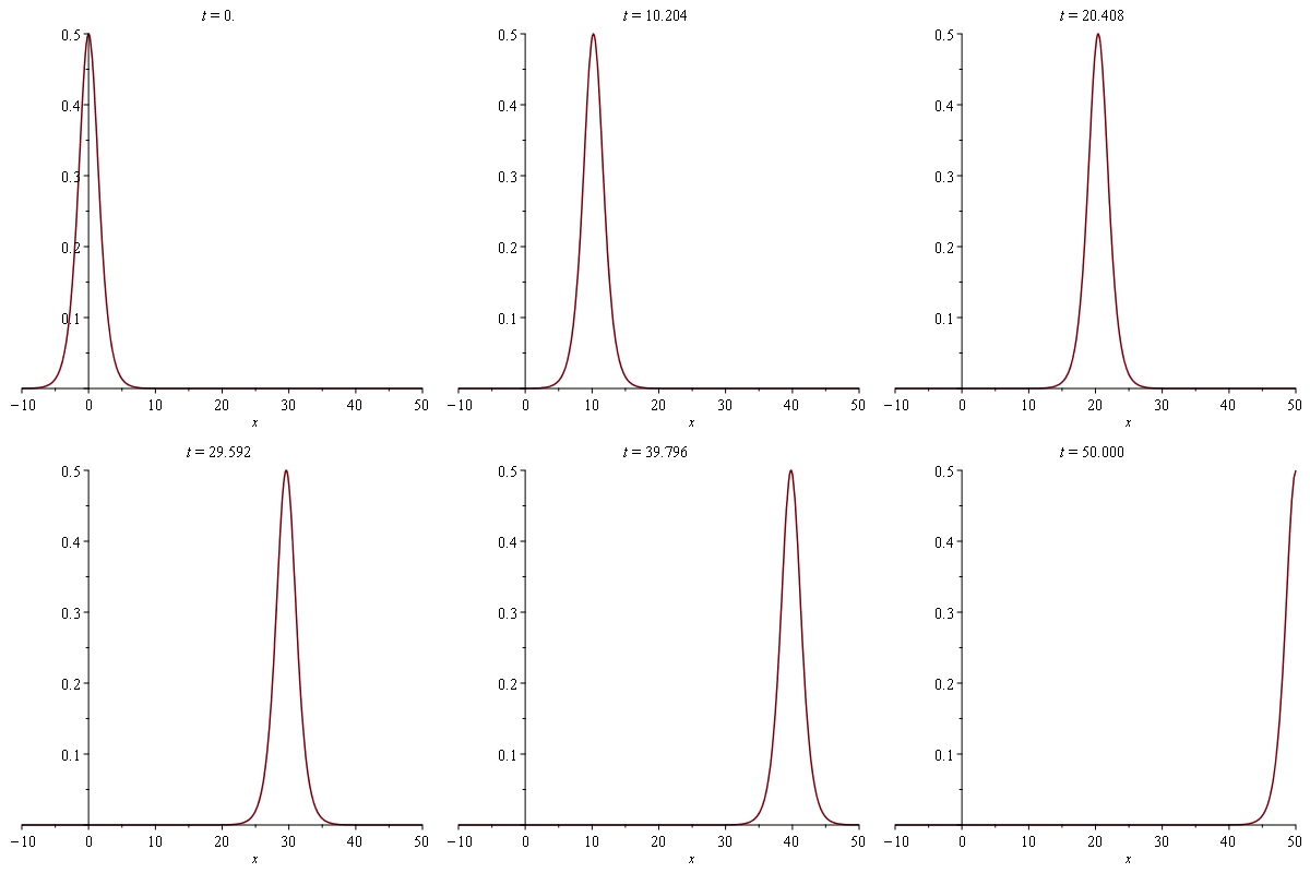
>	plots[animate]( plot, [{sol_example}, x=-10..50], t=0..50, frames=50);

 

>	ODE:=eval(eval(PDE, u(x,t)=f(x-c*t)), x-c*t=xi);

 

(39)

 

>	ODE:=convert(ODE,diff);

 

(40)

 

>	simpler_ODE:=int(lhs(ODE),xi)-A=0;

 

(41)

 

>	sols:=dsolve(simpler_ODE,f(xi)); # There are many solutions and they are not simple

 

(42)

 

Let's give up on analytical solutions and just use numerics to explore our special soliton solutions...next class 

>