What constitutes a “Bayesian” method in deep learning?

First and foremost, it is crucial to understand that all approximate Bayesian inference procedures are non-Bayesian in various ways — otherwise they would not be providing approximate inference. Furthermore, all Bayesian inference procedures in deep learning are approximate, since the posterior predictive distribution cannot be evaluated in closed form (unlike, for example, in Gaussian process regression). Therefore it makes no sense to characterize an approximate inference procedure as fully “Bayesian” or “non-Bayesian”, despite many papers quite arbitrarily dividing the literature in such ways. Instead, each method places somewhere on a spectrum, representing how it approximates the Bayesian ideal. It only makes sense to compare how different approaches place relative to one another on this spectrum. As we will see, deep ensembles are often closer to the Bayesian ideal than many canonical approximate Bayesian inference procedures in deep learning.

In other words, procedures that are being regularly called “Bayesian” are providing lower fidelity Bayesian inference than methods being called “non-Bayesian”, which is particularly problematic when the success of these “non-Bayesian” methods is being used as evidence that we should not pursue “Bayesian methods”. If anything, the “take home message” should be the exact opposite!

Bayesian inference for neural networks

Now let’s step back and understand what we are trying to compute from a Bayesian perspective. In the Bayesian approach, we typically wish to compute the posterior predictive distribution

where \(y\) is an output (e.g., a class label), \(x\) is an input (e.g., an image), \(w\) are parameters, and \(\mathcal{D}\) is the data. This integral forms a Bayesian model average: rather than use a single model corresponding to a single setting of parameters, we wish to average many models corresponding to different parameter settings, weighted by their posterior probabilities.

It is typical to approximate this integral using simple Monte Carlo,

Within the simple Monte Carlo approximation, there are two standard approaches to approximating samples from the posterior: (1) MCMC, and (2) deterministic approaches, such as the Laplace approximation, or variational methods, which approximate the posterior, and then sample from that approximate posterior. The Laplace approximation is constrained to use a Gaussian approximation to the posterior. In practice, variational methods typically also use a Gaussian approximate posterior, for convenience.

Deep ensembles as numerical integration

In deep learning, the integral we are trying to compute is over a multi-million dimensional parameter space, and the posterior is highly non-Gaussian and multi-modal. Moreover, for computational reasons, we are typically limited to about 10-100 points in the parameter space that we can evaluate to form our approximation to the posterior. In this context, it is especially powerful to view approximate inference as numerical integration. From this perspective we want to select for two key properties in our approach to form a good approximation: (i) we would want to find typical points in the posterior, representing regions where there is a lot of mass; (ii) we would also want a diversity of points, such that the different parameters we select give rise to different functions.

Deep ensembles nicely match these desiderata: by re-training our neural network multiple times with different initializations, we typically find different low loss solutions in different basins of attraction, corresponding to a variety of different functions. If we use SGD, these points are not often just low loss, but “typical points”, centred in large basins of attraction. It’s hard to imagine a simple algorithm which would much better approximate our Bayesian posterior predictive distribution under these constraints.

Note that it is also possible to view deep ensembles as forming a posterior approximated as point masses at different modes, combined with a simple Monte Carlo integration: with this posterior, the Bayesian predictive distribution is \(p(y|x, D) = 1/J \sum p(y|x, w_j)\) where \(w_j\) represent the different ensemble weights, which is exactly the standard deep ensemble procedure [1, 3, 8]. Overall, however, we believe the numerical integration perspective is generally more enlightening for why deep ensembles provide a good approximation to the Bayesian predictive distribution [1].

In particular, we emphasize that the points that we select for integral approximation do not have to represent samples from the posterior! Indeed, from the perspective of numerical integration under severe computational constraints, we would not even likely want exact samples from the posterior distribution! If we’re only taking a handful of samples, we don’t want to risk low-density or redundant points. We can also see why standard deterministic approximations with Gaussian approximate posteriors, such as Laplace, and often variational methods, would not provide as good of an approximation to the posterior predictive distribution as deep ensembles: parameter samples from a single basin of attraction typically give very similar models, and thus, unlike deep ensembles, each sample does not provide a good contribution to the integral.

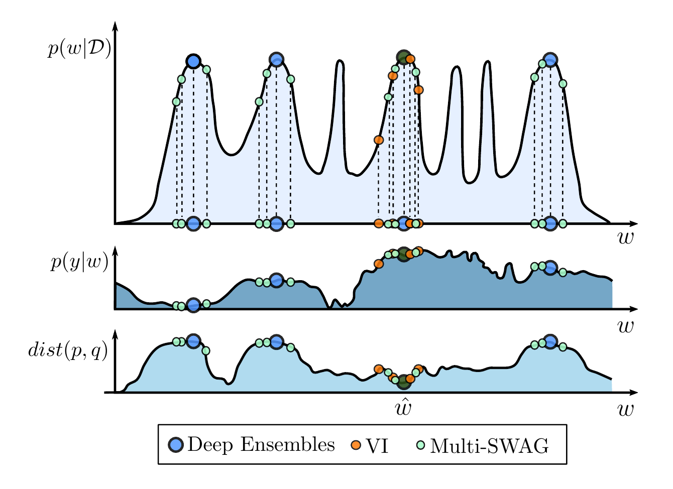
Figure 1. \(p(y|x, D) = \int p(y|x, w)p(w|D)dw\). Top: \(p(w|D)\), with representations from VI (orange) deep ensembles (blue), MultiSWAG (red). Middle: \(p(y|x, w)\) as a function of \(w\) for a test input \(x\). This function does not vary much within modes, but changes significantly between modes. Bottom: Distance between the true predictive distribution and the approximation, as a function of representing a posterior at an additional point \(w\), assuming we have sampled the mode in dark green. There is more to be gained by exploring new basins, than continuing to explore the same basin.

We illustrate this idea conceptually in Figure 1 from [1]. In the top panel, we have a multimodal posterior. In the middle panel, we see the predictive distribution \(p(y|x,w)\) conditioned on parameters \(w\). Within a single basin, the predictive distribution does not change very much, but between basins it is quite different. We would therefore like to select for different basins of attraction in providing a good approximation to the Bayesian model average integral. It is helpful in this context to think of approximate Bayesian inference as an active learning problem: given what we have observed of the posterior so far, where should we go next in order to best improve our approximation of the integral? In this sense, we see clearly that “where we should go next” should not necessarily be defined even by an exact sample from the posterior. In the bottom panel, we see how much we decrease the distance between the true Bayesian predictive distribution \(p\), and our approximation \(q\) by selecting a point in \(w\) space, having observed the point in dark green. We see in this instance we benefit most by selecting other modes.

A remark about simple Monte Carlo integration

In general, the way we view Bayesian inference has become deeply entangled with simple Monte Carlo integration, to the point where it is sometimes treated as synonymous with Bayesian inference, even though it is just one of many possible ways to approximate the Bayesian posterior predictive distribution. Even for an arbitrarily accurate or exact representation of the posterior predictive, there is no need to take posterior samples. Arguably, simple Monte Carlo is a relatively weak way of approximating the posterior predictive (see, for example, Bayesian quadrature [6,7]), despite its convenience, and being the “best of many bad options” in some instances. See [1] for further discussion.

Deep ensembles provide a good approximation of the posterior predictive in practice

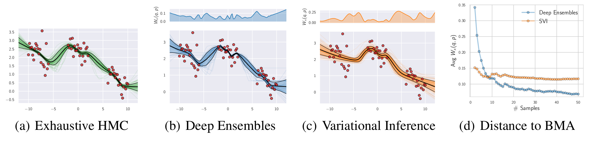
Figure 2. (a): A close approximation of the true predictive distribution obtained by combining 10 HMC chains, each producing 500 samples. (b): Deep ensembles predictive distribution using 50 independently trained networks. (c): Predictive distribution for factorized variational inference (VI). (d): Convergence of the predictive distributions for deep ensembles and variational inference as a function of the number of samples; we measure the average Wasserstein distance between the marginals in the range of input positions. The multi-basin deep ensembles approach provides a more faithful approximation of the Bayesian predictive distribution than the conventional single-basin VI approach, which is overconfident between data clusters. The top panels show the Wasserstein distance between the true predictive distribution and the deep ensemble and VI approximations, as a function of inputs \(x\). For experimental details, see [1].

In Figure 2, we consider a simple regression problem from [1], with three different approximations to the Bayesian predictive distribution: an HMC reference, a variational approximation with a Gaussian approximate posterior, and deep ensembles. For the HMC reference, we run 10 HMC chains, each producing 500 samples; we follow the guidelines described in [2] in setting the parameters of HMC. Further details are in [1].

We measure the Wasserstein divergence between the deep ensemble and the gold standard HMC reference as a function of number of samples in the variational approximation, and number of ensemble components in the deep ensemble. We see that samples from within a single basin, in the variational approximation, provide a very minimal contribution to the integral, because these weights give rise to neural networks that are largely homogenous. On the other hand, additional ensemble components in the deep ensemble greatly improve the fidelity of the approximation to the HMC reference. These results are in-line with our expectations: the value in going between different basins of attraction will be greater for approximating the Bayesian posterior predictive distribution than taking many samples from a single basin, which is the approach provided by most canonical approximate inference procedures.

There has since been exhaustive empirical evidence that deep ensembles do a good job of approximating the Bayesian predictive distribution. In [2], Hamiltonian Monte Carlo procedures are distributed over hundreds of TPUs, to investigate the fundamental properties of neural network posteriors. As part of this study, the authors compare how closely a variety of approximate inference procedures match the posterior predictive distribution of the HMC gold standard, as in Figure 3. We see that deep ensembles are much closer than mean-field variational inference to the HMC reference, and are even comparable to SGLD.

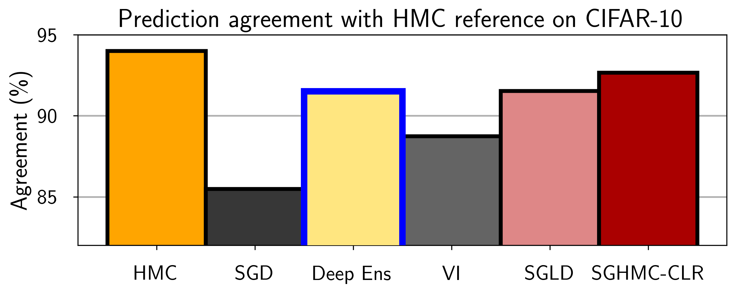
Figure 3. Agreement between predictive distributions of HMC and approximate inference methods: deep ensembles, mean field variational inference (MFVI), and stochastic gradient Monte Carlo (SGMCMC) variations. For all methods we use ResNet-20-FRN trained on CIFAR-10 and evaluate predictions on the CIFAR-10-C test sets and report the average results across all corruptions and corruption intensities. We additionally report the results for HMC for reference: we compute the agreement between one of the chains and the ensemble of the other two chains. Deep ensembles significantly outperform MFVI and perform similarly to SG-MCMC methods in approximating the predictive distribution of HMC. For experimental details, see [2].

What do we gain from understanding deep ensembles as approximate Bayesian inference?

So what can we gain by understanding the connections between deep ensembles and approximate Bayesian inference? This is decidedly not an instance of “everything works because it’s Bayesian”. This perspective provides several conceptually important and actionable takeaways, and prevents a problematic and arbitrary division of the literature. As we summarized at the beginning:
- There are no exact inference procedures in Bayesian deep learning. They are all approximate. Each approximate inference procedure falls onto a spectrum of how closely it matches exact inference. On this spectrum, deep ensembles are typically closer to the Bayesian ideal than many canonical approximate inference procedures, such as mean-field variational inference, and the Laplace approximation.
- In this light, claims that deep ensembles are “non-Bayesian” competitors to many standard approximate inference procedures in Bayesian deep learning are nonsensical. The way the literature is being divided into “Bayesian” and “non-Bayesian” approaches is arbitrary and problematic. If method A is called “non-Bayesian” and method B is called “Bayesian”, but it turns out that method A is actually a better approximation to the Bayesian predictive distribution then method B, then the relative success of method A should not be used as evidence that we should not pursue Bayesian approaches in deep learning.
- Viewing deep ensembles as approximate Bayesian inference provides an actionable mechanism for improving the fidelity of approximate inference. For example, the MultiSWAG procedure [1], which performs Bayesian integration across and within basins of attraction, was directly inspired by this perspective, and provides improved performance over deep ensembles. In general, although deep ensembles provide a high-fidelity approximation to the Bayesian predictive distribution relative to standard approaches, there are also many obvious steps one can take to move deep ensembles closer to a fully Bayesian approach. Moreover, the view of forming the Bayesian predictive distribution as numerical integration rather than obtaining samples for simple Monte Carlo estimation opens the doors to many fresh approaches to approximate inference, lending itself naturally to an active learning perspective.

Now it is true that deep ensembles were not initially motivated as a Bayesian approximation. It is also perfectly valid to derive inspiration from wherever we can find it. Indeed much of early machine learning was inspired by ideas of how the brain works, even though it would be quite a stretch to say that current ML algorithms behave like the human brain. There will also continue to be reasons that deep ensembles in various ways diverge from the Bayesian ideal --- after all, this is true of any approximate inference procedure. But we must be careful not to propagate a false narrative, arbitrarily dividing the literature into “Bayesian” vs “non-Bayesian” approaches, and terming deep ensembles as “non-Bayesian” for reasons that would exclude virtually every procedure described as “Bayesian” in the same paper. We still have to respect reality in framing our research. And the reality is that deep ensembles in practice provide better approximate Bayesian inference in deep learning than many canonical procedures, including mean-field variational inference, and the Laplace approximation, which has recently had a resurgence of popularity as a “Bayesian deep learning” method.

Should we make deep ensembles more Bayesian?

Although deep ensembles represent a relatively high fidelity approximation to the Bayesian posterior predictive distribution in practice, it is perfectly reasonable to further improve the approximation. Indeed, inspired by understanding how deep ensembles perform approximate Bayesian inference, MultiSWAG [1] is one clear way to further improve the approximation, by marginalizing within basins of attraction. We can also use this understanding to move towards more active learning inspired approaches to approximate inference. Since deep ensembles perform approximate inference, there are many ways in which deep ensembles do not perfectly live up to a Bayesian ideal, as with any Bayesian inference procedure in deep learning. We just have to take care not to arbitrarily divide the literature.

There are also cases where a higher fidelity approximation to Bayesian model averaging could be harmful to generalization performance. In particular, [9] shows how deep ensembles can provide better generalization than exact Bayesian model averaging in situations where train and test points are drawn from closely related but different distributions.

There have been many attempts to rationalize “why deep ensembles aren’t Bayesian”. Because deep ensembles represent approximate inference, there are valid ways in which they will differ from the Bayesian ideal. Indeed, many of the claims simply amount to saying that deep ensembles are not providing exact inference. But since any Bayesian inference procedure in deep learning is approximate, it is ill-posed to characterize deep ensembles as “non-Bayesian” for such a reason: one could use a similar approach to disqualify any approximate inference procedure from being called “Bayesian”. Moreover, many of the reasons given are erroneous, or would exclude methods that are being referred to as “Bayesian” in the very same papers, or other papers by the same authors.

We will address many of the common examples and confusions below in a Q&A format. These are all actual claims people have made. There is a non-exhaustive list of possible rationalizations for deep ensembles being “non-Bayesian”. If the underlying reason for making such a claim is not related to good science --- for example, there could be a perception that it might help “sell” the story of a paper, or there could be a resistance to updating one’s beliefs in light of new information (something we must all be familiar with in responding to reviewers), or some form of tribalism in how these methods are viewed --- then of course correcting any one of these claims in isolation could easily just lead to different but equally erroneous new rationalizations. The hope is that by amassing many of these claims, and addressing them in batch, as below, and clearly explaining the general issues with the framing of this discussion, as above, we can finally put to rest the false narrative that deep ensembles are a “non-Bayesian” competitor to standard approximate inference procedures in deep learning.

(1) Claim: Deep ensembles do “model combination” instead of “Bayesian model averaging”.

Response: This confusion likely arises as a result of a (beautifully constructed) note by Tom Minka called “Bayesian model averaging is not model combination”. The note correctly argues that some ensemble methods work by enriching the hypothesis space, whereas Bayesian model averaging simply represents an inability to distinguish between different hypotheses given limited data. As we collect more data, the model average collapses onto a single model.

But what we call “deep ensembles” does not enrich the hypothesis space. They are a strict subset of a full Bayesian model average. Deep ensembles work by maximizing the posterior with SGD several times with different initializations, and then averaging the resulting models. As the posterior collapses onto a single model as it becomes more well defined (e.g., through more data), so does the deep ensemble [1]. The deep ensemble is a posterior weighted model average.

Curiously, deep ensembles are closer in this way to a fully Bayesian procedure than “MC Dropout”, which is often referred to as a “Bayesian deep learning” method. Indeed, MC Dropout will not collapse to a single model, even if the true Bayesian posterior collapses.

(2) Claim: Deep ensembles aren’t Bayesian because they are an equal average of models.

Response: Part of this objection likely arises by viewing Bayesian model averaging purely through the prism of simple Monte Carlo integration. If we view approximate inference as numerical integration then the idea of needing an “unequal” average of models is absurd. However, even via the simple MC perspective, we would expect deep ensemble models to receive close to an equal weighting: the models represent different SGD solutions, which will have very similar values of the loss, and the posterior will have very similar geometry around these solutions.

(3) Claim: Deep ensembles aren’t Bayesian because they don’t have a prior.

Response: Deep ensembles are ensembles of MAP solutions. By definition, maximum a-posteriori optimization involves a prior. The popular Gaussian priors give rise to L2 regularization. But we can easily use any prior we want. Perhaps this confusion arises by forgetting that we can have priors when we do optimization. This claim is just simply false: deep ensembles do have priors.

(4) Claim: Deep ensembles aren’t Bayesian because they are ensembles of MAP solutions.

Response: If this is your definition of what isn’t Bayesian, then it’s tautologically true. But it would be an odd definition, because we can use MAP solutions to provide a better approximation to the Bayesian predictive distribution than many other standard approximate inference procedures that use single basin approximations. Perhaps those making this claim are more precisely trying to say that deep ensembles aren’t exact inference, but that’s true of any Bayesian inference procedure in deep learning.

(5) Claim: Deep ensembles aren’t Bayesian because they don’t select for a diversity of models.

Response: This claim is somewhat ironic because the success of deep ensembles is largely because they do provide a relatively diverse collection of models compared to the models we would obtain, for example, by sampling from a unimodal MFVI posterior. Moreover, Bayesian approaches do not actively select for a diversity of models.

(6) Claim: Deep ensembles aren’t Bayesian because they don’t converge to the true posterior or predictive distribution in the limit of an infinite number of ensemble components.

Response: It’s true that deep ensembles don’t converge asymptotically. But that’s true of virtually any deterministic approximate inference procedure, including the Laplace approximation and variational methods with virtually any approximating distribution (often Gaussian). These methods do not converge to the posterior with number of samples, either (note here we are not talking about convergence with number of data points, n, where deep ensembles do converge). If deep ensembles aren’t Bayesian for this reason, then we should all stop calling Laplace or variational methods Bayesian, despite the resurgence of papers using the Laplace approximation and calling it “Bayesian deep learning”, and the seminal work on Bayesian neural networks with the Laplace approximation by MacKay. The only approximate inference method that has this sort of asymptotic consistency is MCMC. But in practice we use stochastic MCMC in deep learning, which can be biased, and not have this property. Moreover, even if we could use full batch MCMC, we never get anywhere near the asymptotic regime, and typically just use a handful of samples in practice. If, given computational constraints, deep ensembles are typically more Bayesian than many of the alternatives, then you cannot reasonably classify them as a non-Bayesian method.

(7) Claim: There isn’t a limit you can take with deep ensembles such that you get a perfect representation of the posterior or predictive distribution. This is not true of variational methods, because the variational posterior could in principle have unbounded flexibility. Therefore deep ensembles aren’t Bayesian.

Response: Again, if this is your criterion for what gets to be called “Bayesian”, then you should stop calling the Laplace approximation Bayesian inference. Moreover, the whole point of variational methods is to provide a convenient approximating posterior, which is almost always Gaussian. Indeed if we could work with the exact posterior then we wouldn’t need variational inference. Does this mean almost all variational methods in practice are non-Bayesian?

(8) Claim: When our posterior is unimodal, deep ensembles are a silly posterior approximation.

Response: That’s often true. But deep ensembles would be a silly procedure in that context regardless of whether it’s Bayesian. Unlike Laplace, or many other standard approximate inference procedures, outside of deep learning settings deep ensembles don’t make a lot of sense.

But we are talking here about neural networks, which in practice have highly multimodal posteriors --- in fact, many more modes than we are ever going to find by retraining our model with different initializations. If we generally are worried about covering mass within a mode, then we can simply resolve this issue with MultiSWAG [1], which uses a mixture of Gaussians approximation to the posterior, while retaining the advantages of deep ensembles.

(9) Claim: Deep ensembles do not have good approximation guarantees.

Response: The current absence of theoretical guarantees does not say anything about whether a method in practice provides a good Bayesian approximation. Moreover, in deep learning, we are not aware of any approximate inference procedure that would have good approximation guarantees, except perhaps a narrow range of MCMC methods (typically full batch) run for an asymptotically long period of time.

Acknowledgements: We thank Kyunghyun Cho, Matthew D. Hoffman, Sharad Vikram, Yarin Gal, Jannik Kossen, Sebastian Farquhar, Wesley Maddox, Sanyam Kapoor, Wanqian Yang, Kevin Murphy, Shubhendu Trivedi, Kyle Cranmer, Danilo Rezende, Alex Lyzhov, Andrés Potapczynski, and many others, for helpful discussions.

References

[1] A.G. Wilson, P. Izmailov. Bayesian Deep Learning and a Probabilistic Perspective of Generalization. Advances in Neural Information Processing Systems, 2020.

[2] P. Izmailov, S. Vikram, M.D. Hoffman, A.G. Wilson. What Are Bayesian Neural Network Posteriors Really Like? International Conference on Machine Learning, 2021.

[3] A.G. Wilson. The Case for Bayesian Deep Learning. 2019.

[4] A.G. Wilson. Thread on Deep Ensembles as Approximate Bayesian Inference. 2020.

[5] A.G. Wilson. Examining Critiques in Bayesian Deep Learning. Video. April 2021.

[6] C.E. Rasmussen and Z. Ghahramani. Bayesian Monte Carlo. Advances in Neural Information Processing Systems, 2003.

[7] M. Osborne. Bayesian Gaussian processes for sequential prediction, optimisation and quadrature, PhD Thesis, 2010.

[8] F. Gustafsson, M. Danelljan, T. Schon. Evaluating Scalable Bayesian Deep Learning Methods for Robust Computer Vision. CVPR Workshop, 2020.

[9] P. Izmailov, P. Nicholson, S. Lotfi, A. G. Wilson. Dangers of Bayesian Model Averaging under Covariate Shift. Neural Information Processing Systems, 2021.