Sorry for the lateness of this post, but please don't feel any pressure. The basic idea of this week's assignment is for you to have fun trying various advanced things with ray tracing. Below I list several different things you might want to pursue. Try as many of them as you want, or just do a really bang-up job on one or two of them.
In general, you will probably find that there is a tension between trying to do something that runs in "real time" and producing an amazing gorgeous high quality picture. As I showed in class on Monday evening, there are various things you can do to more or less pursue both goals, such as allowing the ray sampling to be varied (eg: a ray at every pixel versus at every nth pixel).
Over the next day or so I'll be expanding out the sections below. If I get specific requests from any of you on any topic, I'll put more detailed notes and suggestions about those topics. If you have some other specific ray-tracing related topic you want to pursue, let me know and I'll put up notes about that.
If people feel really excited about this topic, we can spend another week on it, since much of the material on surface shading can be learned in the context of a ray tracer, rather than waiting to implement the scan-line renderer that we will cover in several weeks.
Sub-sampling and super-sampling
As some of you have already figured out, you can choose to sub-sample at a lower effective resolution: rather than shooting a ray at every pixel, you can shoot one every 3×3 pixels, or every 4×4 pixels, etc. One interesting possibility, if you're ray tracing to a scene with no moving objects, is to shoot rays at nth pixel while the user is rotating the view. Then when the user stops rotating the view, switch to a higher resolution.
Another possibility is to sub-sample very nth pixel, and then go back and look at where there were large differences in color between two samples. In those places (ie: at visual edges) go back and shoot a ray at every pixel.
You can also choose to super-sample at visual edges: rather than shoot only a single ray at pixels where you detect a large change in color from one pixel to the next, you can shoot 2×2 rays at those pixels, or 3×3 rays, etc. If you do this, then you should offset the aim directions of these rays so that each ray goes through a different part of the pixel. Then you can average the results from these n×<>n rays to get a smoothed or anti-aliased edge.
Ray tracing to generalized second order polynomials
In general you can describe any second order equation in three dimensions (an equation whose terms have polynomial powers of at most two) by ten terms:
ax2 + by2 + cz2 + dyz + ezx + fxy + gx + hy + iz + j = 0In this way you can describe any ellipsoid, paraboloid or hyperboloid surface. This includes spheres as a special case.
In order to ray trace to such surfaces, you would need to substitute [vx+twx, vy+twy, vz+twz] into this equation, which will give you a quadratic equation only in t, which you could then solve.
One interesting question is: once you have found where the ray intersects such a surface, how do you compute the surface normal vector for shading? The answer is that you need to look at the derivative equation, which gives a vector valued gradient at each point:
[ 2ax + ez + fy + g , 2by + dz + fx + h , 2cz + dy + ex + i ]If you evaluate this at your surface point, and normalize it to unit length, you will obtain the normal vector at that surface point (the unit length vector which points perpendicularly out of the surface at that point).
Boolean union, intersection and difference
As we discussed in class (and as one or two of you have already implemented) you can do boolean unions, intersections and differences along each ray to create composite objects.
The trick to developing a general boolean object is to maintain a list of "hits" of the ray with surfaces that it encounters, which should always remain sorted in order of increasing t. You then need to be able to combine those lists with union, intersection and difference operators.
Each item on this list should contain the following data fields: [t, surfaceId, sign = +1 or -1]. Their respective meanings are as follows:
A OR B = ¬ ( ¬A AND ¬B )
A - B = A AND ¬B
Ray tracing to polyhedra
First, let's define a half-space (a,b,c,d) by its characteristic equation ax+by+cz+d≥0. In other words, this half-space consists of those points (x,y,z) such that ax+by+cz+d≥0. Notice that the half-space is bounded by the plane ax+by+cz+d=0.
Here's a simple observation: If you can ray trace to a plane, then you can ray trace to any convex polyhedron, since a convex polyhedron can be defined as an intersection of planes.
To trace ray [vx+twx, vy+twy, vz+twz] to half-space ax+by+cz+d≥0 you just need to substitute for x, y and z:
a(vx+twx) + b(vy+twy) + c(vz+twz) + d ≥ 0and solve for t. This will give you a boolean list with at most one item on it.
To intersect the ray with the entire polyhedron, just intersect the ray with each of its constituent half-spaces, and can call your ∧ operator on all the results.
When it comes time to do shading, you'll need a normal vector. As always, you can obtain this by taking the vector-valued derivative, or "gradient", of the half-space's characteristic equation. To do this, you take the three partial derivatives, in x, y and z, respectively, of ax+by+cz+d. These are, respectively, a, b and c. Therefore, the gradient is just the constant vector [a,b,c]. If you normalize this vector to unit length you obtain the surface normal vector.
Shadows
We already discussed this somewhat last week, but I'll review. Once your ray has hit that first visible surface point, which we can refer to as s = (sx,sy,sz), the key is to create another ray that goes from s into the direction of the light vector L, and see whether that ray intersects anything.
If this shadow ray hits anything, then the surface point is in shadow, and should only be illuminated by the ambient color. If the shadow ray doesn't hit anything, then the surface point should be fully illuminated by that light source.
When you shoot this ray, one danger is that your ray tracer will accidentally find the surface point s itself, due to numerical inaccuracies. You don't want that. To avoid this, the trick that I usually use is to use, as the origin of the shadow ray, not exactly s itself, but a point that's already been moved a little bit along the ray by some small distance ε. So your ray should actually be defined by v+tw, where: v = s+εL and w = L.
Shiny hilights and phong shading
Up till now all your surfaces have looked dull, lifeless, boring, blah. That's because we didn't put any highlights on them. One cool thing about highlights is that, in addition to being all bright an shiny, they change as the object moves. In this way, highlights provide useful visual information about shape and motion.
The simplest model for approximating surface highlights is the Phong model, originally developed by Bui-Tong Phong. In this model, we think of the interaction between light and a surface as having three distinct components:
The diffuse component is that dot product n•L that we discussed in the previous assignment. It approximates light, originally from light source L, reflecting from a surface which is diffuse, or non-glossy. One example of a non-glossy surface is paper. In general, you'll also want this to have a color value, so this term would in general be a color defined as: [rd,gd,bd](n•L).
Finally, the Phong model has a provision for a highlight, or specular, component, which reflects light in a shiny way. This is defined by [rs,gs,bs](R•L)p, where R is the mirror reflection direction vector we defined in the previous assignment, and where p is a specular power. The higher the value of p, the shinier the surface.
The complete Phong shading model for a single light source is:
[ra,ga,ba] + [rd,gd,bd](n•L) + [rs,gs,bs](R•L)p
If you have multiple light sources, the effect of each light source Li will geometrically depend on the normal, and therefore on the diffuse and specular components, but not on the ambient component. Also, each light might have its own [r,g,b] color. So the complete Phong model for multiple light sources is:
[ra,ga,ba] + Σi( [Lr,Lg,Lb] ( [rd,gd,bd](n•Li) + [rs,gs,bs](R•Li)p ) )
If you have multiple light sources,
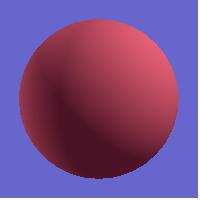
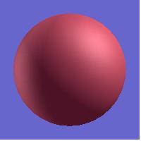
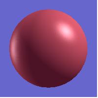
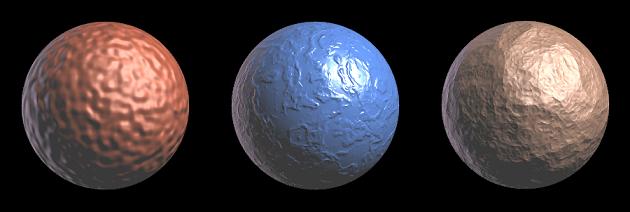
Below you can see three different shaders for a sphere. In all cases, the sphere is lit by two light sources: a dim source from the rear left (-1,0,-.5) and a bright source from the front upper right (1,1,.5). The spheres have, respectively, no highlight, a highlight with an exponent of p = 4, and a highlight with an exponent of p = 16.
Reflections
Mirror reflections are pretty straightforward in ray tracing. You just compute the reflection angle, as I described in the notes for the first ray tracing assignment, and then you continue the ray from there. Generally you get the most realistic (and nicest looking) effect if you assume that only some portion of the surface reflectance is mirror reflecting, and the rest is modeled by some sort of light-scattering model, such as is approximated by the Phong algorithm. In other words, whatever color you get back from shooting your mirror-reflection ray, you can mix together in some proportion with a Phong calculation.
One thing that's really cool is to combine mirror reflections with the sort of procedural bump textures that I describe below. This combination is sure to impress friends, relatives and graphics professors.
Transparency and refraction
In addition to a ray of light bouncing off a surface, some of the light might actually go through the surface. This can happen, for example, if light encounters such transparent materials as glass or water or lucite. When this happens in nature, there is generally refraction, or bending of light where the ray enters or leaves the transparent material.
Refraction is governed by Snell's Law, which states that light will bend in a way that is determined by the material's index of refraction, or n, which indicates how much more slowly the light travels in this medium, in comparison with the speed of light in a vacuum. For example, light travels through a material with an index of refraction of n=1.5 at a speed of 1/1.5, or 2/3 of the speed of light in a vacuum.
The speed of light through air is so close to the speed of light in a vacuum that we can pretty much approximate its index of refraction by n=1. The index of refraction of glass is typically around n=1.4.
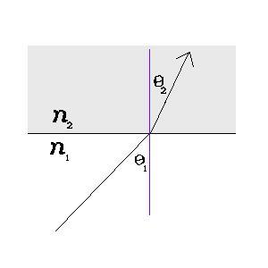
Specifically, Snell's Law states that if an incoming ray travelling through a medium that has an index of refraction of n1 crosses over into another medium that has an index of refraction of n2, then the relationship between the angle θ1 by which the entering ray deviates from the surface normal, and the angle θ2 by which the exiting ray deviates from the surface normal, is given by n1 sinθ1 = n2 sinθ2 .
Atmosphere: fog, pea soup, etc.
In the presence of fog, objects gradually fade from view, as a function of their distance from your eye. In the case of uniform fog (ie: fog with the same density everywhere), it is pretty easy to model and render this effect. The key observation is that for any uniform fog there is some distance D that a beam light has to travel before half of the light in the beam has been scattered away by fog particles. The other half of the light continues along the beam unobstructed.
Now consider what happens when the light which has made it through the fog travels further by another distance D. Half of the remaining light will now be scattered away, and half of the remaining light will make it through the second distance. In other words, the light that makes it through a distance 2D unobstructed is (1/2)2. And in general, the amount of light that makes it through a distance kD is (1/2)k, for any value of k.
To calculate uniform fog which scatters half of its light every distance D, you need to measure the distance d traveled by the ray (ie: the distance from the ray origin to the surface point that the ray hits). The proportion of this light that makes it through the fog unscattered will be t=(1/2)d/D. The effect of the fog can be shown by mixing t(surfaceColor) + (1-t)(fogColor), where surfaceColor is the color that you would have calculated had there been no fog. Some uniform shade of light gray, such as (0.8,0.8,0.8), generally works well for the fog color.
Bumpy surfaces, Noise, procedural textures
In order to make a surface appear bumpy, it is not necessary to actually put little hills and valleys in the surface. Instead, we can modify the surface normal vector, to give the impression of a bumpy surface, as I discussed in class. It turns out that this is a lot less computationally expensive. This basic trick was first developed by Jim Blinn around 1977.
The example of bump mapping that I showed in class (somewhat improved) is at:
You can grab my reference noise implementation from http://mrl.nyu.edu/~perlin/noise/
How to transform a general quadratic equation in three dimensions
As I pointed out in the last class, plane equation ax + by + cz + d, which characterizes the plane p containing points xT, can be defined by the following dot product:
(a b c d) • x
y
z
1= 0
or, in other words, p xT = 0. This makes it clear that if you want to find the plane that contains transformed points M•xT, then you need to replace p with p M-1.
Similarly, we can define quadratic equation
ax2 + by2 + cz2 + dyz + ezx + fxy + gx + hy + iz + j = 0by the following double dot product:
(x,y,z,1) • a f e g
0 b d h
0 0 c i
0 0 0 j• x
y
z
1= 0
or in other words, x P xT = 0, where P denotes the 10 quadratic coefficients arranged into the above 4×4 matrix.
This means that if you want to find the three-variable quadratic equation that contains transformed points M•xT, you need to replace P by (M-1)T P M-1, because that will give you:
(M xT)T (M-1)T P M-1 (M xT) =
xT MT (M-1)T P M-1 M xT =
x P xT = 0